외부 응용 프로그램 환경 설정¶

윈도우 사용자를 위한 소고
파일 포맷에 대한 소고
벡터 레이어 선택에 대한 소고
SAGA
R scripts
- Adding R scripts from the QGIS collection
- Creating R scripts
R libraries
- R libraries installed when running sf_test
GRASS
LAStools

The processing framework can be extended using additional applications. Algorithms that rely on external applications are managed by their own algorithm providers. Additional providers can be found as separate plugins, and installed using the QGIS Plugin Manager.

This section will show you how to configure the Processing framework to include these additional applications, and it will explain some particular features of the algorithms based on them. Once you have correctly configured the system, you will be able to execute external algorithms from any component like the toolbox or the graphical modeler, just like you do with any other algorithm.

By default, algorithms that rely on an external application not shipped with QGIS are not enabled. You can enable them in the Processing settings dialog if they are installed on your system.

윈도우 사용자를 위한 소고 ¶

If you are not an advanced user and you are running QGIS on Windows, you might not be interested in reading the rest of this chapter. Make sure you install QGIS in your system using the standalone installer. That will automatically install SAGA and GRASS in your system and configure them so they can be run from QGIS. All the algorithms from these providers will be ready to be run without needing any further configuration. If installing with the OSGeo4W application, make sure that you also select SAGA and GRASS for installation.

파일 포맷에 대한 소고 ¶

When using external software, opening a file in QGIS does not mean that it can be opened and processed in that other software. In most cases, other software can read what you have opened in QGIS, but in some cases, that might not be true. When using databases or uncommon file formats, whether for raster or vector layers, problems might arise. If that happens, try to use well-known file formats that you are sure are understood by both programs, and check the console output (in the log panel) to find out what is going wrong.

You might for instance get trouble and not be able to complete your work if you call an external algorithm with a GRASS raster layers as input. For this reason, such layers will not appear as available to algorithms.

You should, however, not have problems with vector layers, since QGIS automatically converts from the original file format to one accepted by the external application before passing the layer to it. This adds extra processing time, which might be significant for large layers, so do not be surprised if it takes more time to process a layer from a DB connection than a layer from a Shapefile format dataset of similar size.

외부 응용 프로그램을 사용하지 않는 제공자는, QGIS를 통해서 레이어를 열어 분석하기 때문에 QGIS가 열 수 있는 모든 레이어를 처리할 수 있습니다.

All raster and vector output formats produced by QGIS can be used as input layers. Some providers do not support certain formats, but all can export to common formats that can later be transformed by QGIS automatically. As for input layers, if a conversion is needed, that might increase the processing time.

벡터 레이어 선택에 대한 소고 ¶

외부 응용 프로그램이 QGIS 안에 존재하는 벡터 레이어 선택 집합을 인지하게 만들 수도 있습니다. 하지만 원본 벡터 레이어들이 외부 응용 프로그램이 지원하지 않는 포맷인 경우, 이렇게 하려면 모든 입력 벡터 레이어를 재작성해야만 합니다. 어떤 선택 집합도 없을 때만, 또는 공간 처리 일반 환경 설정에서 |unchecked| Use only selected features 옵션이 비활성화된 경우에만 외부 응용 프로그램으로 레이어를 직접 넘겨줄 수 있습니다.

In other cases, exporting only selected features is needed, which causes longer execution times.

SAGA ¶

SAGA algorithms can be run from QGIS if SAGA included in the QGIS installation.

If you are running Windows, both the stand-alone installer and the OSGeo4W installer include SAGA.

SAGA 그리드 시스템 제약에 관해 ¶

입력 래스터 데이터 여러 개를 요구하는 SAGA 알고리즘 대부분은 입력 래스터가 동일한 그리드 시스템을 보유하고 있을 것을 요구합니다. 즉, 입력 래스터들이 동일한 지리 영역을 커버하고 동일한 셀 크기를 가지고 있어야만 하기 때문에 그에 대응하는 그리드들도 일치해야만 한다는 뜻입니다. QGIS에서 SAGA 알고리즘을 호출하는 경우 사용자는 셀 크기나 범위에 상관없이 어떤 레이어든 사용할 수 있습니다. SAGA 알고리즘이 여러 래스터 레이어를 입력받아야 한다면 (해당 알고리즘이 서로 다른 그리드 시스템을 가진 레이어들을 처리할 수 없는 경우) QGIS가 래스터들을 공통 그리드 시스템으로 리샘플링해서 SAGA에 넘겨줍니다.

이때 공통 그리드 시스템은 사용자가 정의합니다. 설정 대화창에서 SAGA 그룹에 있는 파라미터 몇 가지를 사용해서 정의할 수 있습니다. 다음 두 가지 방법 가운데 하나로 대상 그리드 시스템을 설정합니다:

직접 설정합니다. 다음 파라미터의 값을 설정해서 범위를 정의합니다:
- Resampling min X
- Resampling max X
- Resampling min Y
- Resampling max Y
- Resampling cellsize
설정한 범위와 입력 레이어의 범위가 일치하지 않더라도 QGIS가 입력 레이어들을 설정한 범위로 리샘플링할 것이라는 사실을 유념하십시오.
입력 레이어로부터 자동 설정합니다. 이 옵션을 선택하려면, |checkbox| Use min covering grid system for resampling 옵션을 체크하면 됩니다. 다른 모든 설정을 무시하고 모든 입력 레이어를 커버하는 최소 범위를 사용할 것입니다. 대상 레이어의 셀 크기는 입력 레이어들의 모든 셀 크기 가운데 가장 큰 크기를 사용합니다.

여러 래스터 레이어를 사용하지 않는 알고리즘의 경우, 또는 유일한 입력 그리드 시스템을 요구하지 않는 알고리즘의 경우 SAGA 호출 전에 리샘플링을 하지 않으므로 이런 파라미터들도 사용하지 않습니다.

다중 밴드 레이어에 대한 제약 ¶

QGIS와 달리, SAGA는 다중 밴드 레이어를 지원하지 않습니다. (RGB 또는 다중 스펙트럼 이미지 같은) 다중 밴드 레이어를 사용하고 싶다면 먼저 해당 레이어를 단일 밴드 이미지로 분할해야 합니다. RGB 이미지에서 이미지 3개를 생성하는 SAGA/Grid - Tools/Split RGB image 알고리즘을 사용하거나 또는 단일 밴드 이미지를 추출하는 SAGA/Grid - Tools/Extract band 알고리즘을 사용하면 됩니다.

셀 크기에 대한 제약 ¶

SAGA는 래스터 레이어의 X 및 Y 방향의 셀 크기가 동일하다고 가정하고 있습니다. 수평 및 수직 셀 크기가 다른 레이어를 작업하는 경우, 기대하지 않은 결과물이 나올 수도 있습니다. 이런 경우, SAGA가 처리하기에 적합하지 않은 입력 레이어일 수도 있다는 경고 메시지가 공간 처리 로그에 추가될 것입니다.

로그 작업 ¶

QGIS가 SAGA를 호출할 때 SAGA 명령 줄 인터페이스를 사용해서 필요한 모든 작업을 수행하기 위한 명령어 집합을 넘겨줍니다. SAGA는 그 진행 상태를 콘솔에 정보를 작성해서 표시하는데, 이 정보는 이미 완료된 공간 처리 작업의 백분율 및 부가적인 내용을 포함합니다. 알고리즘 실행 도중 이 산출 정보를 필터링해서 진행 상태 막대를 업데이트합니다.

Both the commands sent by QGIS and the additional information printed by SAGA can be logged along with other processing log messages, and you might find them useful to track what is going on when QGIS runs a SAGA algorithm. You will find two settings, namely Log console output and Log execution commands, to activate that logging mechanism.

Most other providers that use external applications and call them through the command-line have similar options, so you will find them as well in other places in the processing settings list.

R scripts ¶

To enable R in Processing you need to install the Processing R Provider plugin and configure R for QGIS.

Configuration is done in Provider-> R in the Processing tab of Settings-> Options.

Depending on your operating system, you may have to use R folder to specify where your R binaries are located.

참고

On Windows the R executable file is normally in a folder (R-<version>) under C:\Program Files\R\. Specify the folder and NOT the binary!

On Linux you just have to make sure that the R folder is in the PATH environment variable. If R in a terminal window starts R, then you are ready to go.

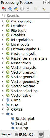
After installing the Processing R Provider plugin, you will find some example scripts in the Processing Toolbox:

Scatterplot runs an R function that produces a scatter plot from two numerical fields of the provided vector layer.
test_sf does some operations that depend on the sf package and can be used to check if the R package sf is installed. If the package is not installed, R will try to install it (and all the packages it depends on) for you, using the Package repository specified in Provider-> R in the Processing options. The default is http://cran.at.r-project.org/. Installing may take some time…
test_sp can be used to check if the R package sp is installed. If the package is not installed, R will try to install it for you.

../../../_images/processing_toolbox_r_install.png

If you have R configured correctly for QGIS, you should be able to run these scripts.

Adding R scripts from the QGIS collection ¶

R integration in QGIS is different from that of SAGA in that there is not a predefined set of algorithms you can run (except for some example script that come with the Processing R Provider plugin).

A set of example R scripts is available in the QGIS Repository. Perform the following steps to load and enable them using the QGIS Resource Sharing plugin.

Add the QGIS Resource Sharing plugin (you may have to enable Show also experimental plugins in the Plugin Manager Settings)
Open it (Plugins-> Resource Sharing-> Resource Sharing)
Choose the Settings tab
Click Reload repositories
Choose the All tab
Select QGIS R script collection in the list and click on the Install button
The collection should now be listed in the Installed tab
Close the plugin
Open the Processing Toolbox, and if everything is OK, the example scripts will be present under R, in various groups (only some of the groups are expanded in the screenshot below).

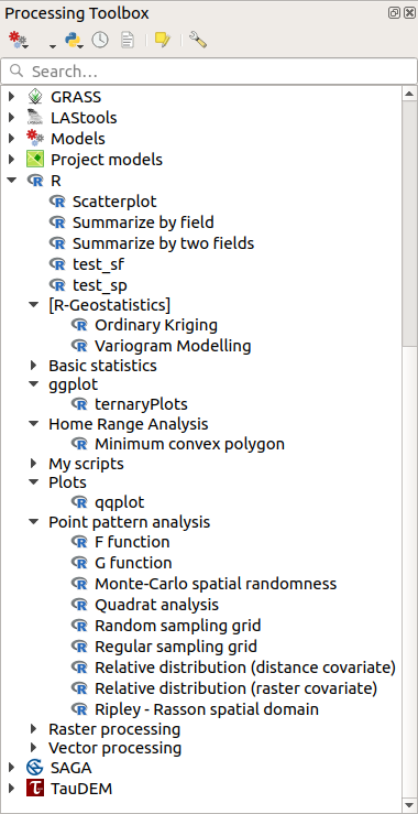
The Processing Toolbox with some R scripts shown¶

The scripts at the top are the example scripts from the Processing R Provider plugin.
If, for some reason, the scripts are not available in the Processing Toolbox, you can try to:
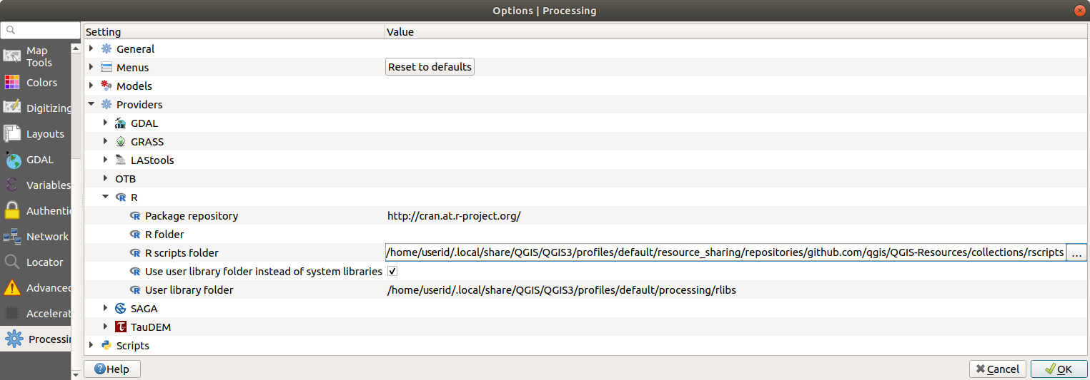
1. Open the Processing settings (Settings-> Options-> Processing tab)
2. Go to Providers-> R-> R scripts folder
  - On Ubuntu, set the path to (or, better, include in the path):
    
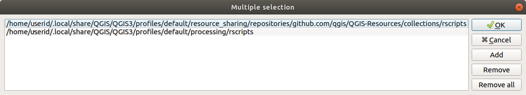
    /home/<user>/.local/share/QGIS/QGIS3/profiles/default/resource_sharing/repositories/github.com/qgis/QGIS-Resources/collections/rscripts
  - On Windows, set the path to (or, better, include in the path):
    
    C:\Users\<user>\AppData\Roaming\QGIS\QGIS3\profiles\default\resource_sharing\repositories\github.com\qgis\QGIS-Resources\collections\rscripts
  To edit, double-click. You can then choose to just paste / type the path, or you can navigate to the directory by using the … button and press the Add button in the dialog that opens. It is possible to provide several directories here. They will be separated by a semicolon (《;》).

If you would like to get all the R scrips from the QGIS 2 on-line collection, you can select QGIS R script collection (from QGIS 2) instead of QGIS R script collection. You will find probably find that scripts that depend on vector data input or output will not work.

Creating R scripts ¶

You can write scripts and call R commands, as you would do from R. This section shows you the syntax for using R commands in QGIS, and how to use QGIS objects (layers, tables) in them.

To add an algorithm that calls an R function (or a more complex R script that you have developed and you would like to have available from QGIS), you have to create a script file that performs the R commands.

R script files have the extension .rsx, and creating them is pretty easy if you just have a basic knowledge of R syntax and R scripting. They should be stored in the R scripts folder. You can specify the folder (R scripts folder) in the R settings group in Processing settings dialog).

Let’s have a look at a very simple script file, which calls the R method spsample to create a random grid within the boundary of the polygons in a given polygon layer. This method belongs to the maptools package. Since almost all the algorithms that you might like to incorporate into QGIS will use or generate spatial data, knowledge of spatial packages like maptools and sp/sf, is very useful.

##Random points within layer extent=name
##Point pattern analysis=group
##Vector_layer=vector
##Number_of_points=number 10
##Output=output vector
library(sp)
spatpoly = as(Vector_layer, "Spatial")
pts=spsample(spatpoly,Number_of_points,type="random")
spdf=SpatialPointsDataFrame(pts, as.data.frame(pts))
Output=st_as_sf(spdf)

The first lines, which start with a double Python comment sign (##), define the display name and group of the script, and tell QGIS about its inputs and outputs.

참고

To find out more about how to write your own R scripts, have a look at the R Intro section in the training manual and consult the QGIS R Syntax section.

When you declare an input parameter, QGIS uses that information for two things: creating the user interface to ask the user for the value of that parameter, and creating a corresponding R variable that can be used as R function input.

In the above example, we have declared an input of type vector, named Vector_layer. When executing the algorithm, QGIS will open the layer selected by the user and store it in a variable named Vector_layer. So, the name of a parameter is the name of the variable that you use in R for accessing the value of that parameter (you should therefore avoid using reserved R words as parameter names).

Spatial parameters such as vector and raster layers are read using the st_read() (or readOGR) and brick() (or readGDAL) commands (you do not have to worry about adding those commands to your description file – QGIS will do it), and they are stored as sf (or Spatial*DataFrame) objects.

Table fields are stored as strings containing the name of the selected field.

Vector files can be read using the readOGR() command instead of st_read() by specifying ##load_vector_using_rgdal. This will produce a Spatial*DataFrame object instead of an sf object.

Raster files can be read using the readGDAL() command instead of brick() by specifying ##load_raster_using_rgdal.

If you are an advanced user and do not want QGIS to create the object for the layer, you can use ##pass_filenames to indicate that you prefer a string with the filename. In this case, it is up to you to open the file before performing any operation on the data it contains.

With the above information, it is possible to understand the first lines of the R script (the first line not starting with a Python comment character).

library(sp)
spatpoly = as(Vector_layer, "Spatial")
pts=spsample(polyg,numpoints,type="random")

The spsample function is provided by the sp library, so the first thing we do is to load that library. The variable Vector_layer contains an sf object. Since we are going to use a function (spsample) from the sp library, we must convert the sf object to a SpatialPolygonsDataFrame object using the as function.

Then we calling the spsample function, with this object and the numpoints input parameter (which specifies the number of points to generate).

Since we have declared a vector output named Output, we have to create a variable named Output containing an sf object.

We do this in two steps. First we create a SpatialPolygonsDataFrame object from the result of the function, using the SpatialPointsDataFrame function, and then we convert that object to an sf object using the st_as_sf function (of the sf library).

You can use whatever names you like for your intermediate variables. Just make sure that the variable storing your final result has the defined name (in this case Output), and that it contains a suitable value (an sf object for vector layer output).

In this case, the result obtained from the spsample method had to be converted explicitly into an sf object via a SpatialPointsDataFrame object, since it is itself an object of class ppp, which can not be returned to QGIS.

사용자 알고리즘이 래스터 레이어를 생성하는 경우, 사용자가 ##dontuserasterpackage 태그를 사용했는지 여부에 따라 래스터를 저장하는 방식이 달라질 것입니다. 해당 태그를 사용했다면, writeGDAL() 메소드를 사용해서 레이어를 저장합니다. 사용하지 않았다면, raster 패키지의 writeRaster() 메소드를 사용할 것입니다.

If you have used the ##pass_filenames option, outputs are generated using the raster package (with writeRaster()).

If your algorithm does not generate a layer, but a text result in the console instead, you have to indicate that you want the console to be shown once the execution is finished. To do so, just start the command lines that produce the results you want to print with the > (〈greater than〉) sign. Only output from lines prefixed with > are shown. For instance, here is the description file of an algorithm that performs a normality test on a given field (column) of the attributes of a vector layer:

##layer=vector
##field=field layer
##nortest=group
library(nortest)
>lillie.test(layer[[field]])

마지막 행의 산출물을 출력하지만, 그 위 행의 산출물은 출력되지 않습니다. (그리고 각 행의 산출물 가운데 어느 쪽도 QGIS에 자동적으로 추가되지 않습니다.)

If your algorithm creates any kind of graphics (using the plot() method), add the following line (output_plots_to_html used to be showplots):

##output_plots_to_html

이 태그를 사용하면, QGIS가 모든 R 그래픽 산출물을 임시 파일로 돌려서, R 실행이 종료된 다음 불러올 것입니다.

Both graphics and console results will be available through the processing results manager.

For more information, please check the R scripts in the official QGIS collection (you download and install them using the QGIS Resource Sharing plugin, as explained elsewhere). Most of them are rather simple and will greatly help you understand how to create your own scripts.

참고

The sf, rgdal and raster libraries are loaded by default, so you do not have to add the corresponding library() commands. However, other additional libraries that you might need have to be explicitly loaded by typing: library(ggplot2) (to load the ggplot2 library). If the package is not already installed on your machine, Processing will try to download and install it. In this way the package will also become available in R Standalone. Be aware that if the package has to be downloaded, the script may take a long time to run the first time.

R libraries ¶

The R script sp_test tries to load the R packages sp and raster.

R libraries installed when running sf_test ¶

The R script sf_test tries to load sf and raster. If these two packages are not installed, R may try to load and install them (and all the libraries that they depend on).

The following R libraries end up in ~/.local/share/QGIS/QGIS3/profiles/default/processing/rscripts after sf_test has been run from the Processing Toolbox on Ubuntu with version 2.0 of the Processing R Provider plugin and a fresh install of R 3.4.4 (apt package r-base-core only):

abind, askpass, assertthat, backports, base64enc, BH, bit, bit64, blob, brew, callr, classInt, cli, colorspace, covr, crayon, crosstalk, curl, DBI, deldir, desc, dichromat, digest, dplyr, e1071, ellipsis, evaluate, fansi, farver, fastmap, gdtools, ggplot2, glue, goftest, gridExtra, gtable, highr, hms, htmltools, htmlwidgets, httpuv, httr, jsonlite, knitr, labeling, later, lazyeval, leafem, leaflet, leaflet.providers, leafpop, leafsync, lifecycle, lwgeom, magrittr, maps, mapview, markdown, memoise, microbenchmark, mime, munsell, odbc, openssl, pillar, pkgbuild, pkgconfig, pkgload, plogr, plyr, png, polyclip, praise, prettyunits, processx, promises, ps, purrr, R6, raster, RColorBrewer, Rcpp, reshape2, rex, rgeos, rlang, rmarkdown, RPostgres, RPostgreSQL, rprojroot, RSQLite, rstudioapi, satellite, scales, sf, shiny, sourcetools, sp, spatstat, spatstat.data, spatstat.utils, stars, stringi, stringr, svglite, sys, systemfonts, tensor, testthat, tibble, tidyselect, tinytex, units, utf8, uuid, vctrs, viridis, viridisLite, webshot, withr, xfun, XML, xtable

GRASS ¶

Configuring GRASS is not much different from configuring SAGA. First, the path to the GRASS folder has to be defined, but only if you are running Windows.

By default, the Processing framework tries to configure its GRASS connector to use the GRASS distribution that ships along with QGIS. This should work without problems for most systems, but if you experience problems, you might have to configure the GRASS connector manually. Also, if you want to use a different GRASS installation, you can change the setting to point to the folder where the other version is installed. GRASS 7 is needed for algorithms to work correctly.

If you are running Linux, you just have to make sure that GRASS is correctly installed, and that it can be run without problem from a terminal window.

GRASS 알고리즘은 계산 시 영역(region)을 사용합니다. SAGA 환경 설정에서와 비슷한 값들을 사용해서 이 영역을 직접 정의할 수도 있고, 또는 알고리즘 실행 시 사용되는 모든 입력 레이어를 커버하는 최소 범위를 받아 자동으로 정의하도록 할 수도 있습니다. 만약 두 번째 습성을 선호한다면, GRASS 환경 설정 파라미터 가운데 |checkbox| Use min covering region 옵션을 체크하면 됩니다.

LAStools ¶

To use LAStools in QGIS, you need to download and install LAStools on your computer and install the LAStools plugin (available from the official repository) in QGIS.

On Linux platforms, you will need Wine to be able to run some of the tools.

LAStools is activated and configured in the Processing options (Settings ‣ Options, Processing tab, Providers‣ LAStools), where you can specify the location of LAStools (LAStools folder) and Wine (Wine folder). On Ubuntu, the default Wine folder is /usr/bin.