.
La boîte à outils
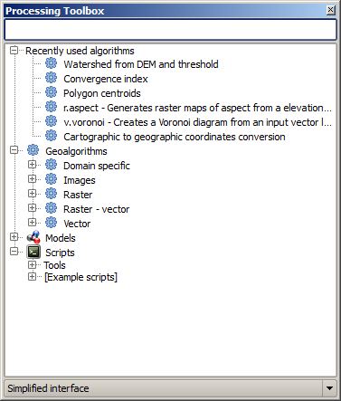
La Boîte à outils est l’élément principal du module de Traitements et probablement celui que vous utiliserez le plus au quotidien. Elle montre la liste des algorithmes disponibles, regroupés en plusieurs catégories. C’est aussi par son intermédiaire qu’il est possible d’exécuter un algorithme sur un jeu de données en entrée, ponctuellement ou par lot.
Figure Processing 5:
Processing Toolbox 
The toolbox contains all the available algorithms, divided into predefined groups. All these groups are found under a single tree entry named Geoalgorithms.
Additionally, two more entries are found, namely Models and Scripts. These include user-created algorithms, and they allow you to define your own workflows and processing tasks. We will devote a full section to them a bit later.
Dans la partie haute de la boîte à outils se trouve un champ texte. Pour réduire le nombre d’algorithmes affichés dans la boîte à outils et vous permettre de trouver celui qui vous convient, il vous suffit d’entrer un mot-clé ou une phrase dnas ce champ. La liste des algorithmes contenant ce texte est filtrée au fur et à mesure de la saisie.
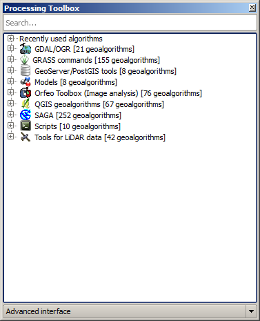
In the lower part, you will find a box that allows you to switch between the simplified algorithm list (the one explained above) and the advanced list. If you change to the advanced mode, the toolbox will look like this:
Figure Processing 6:
Processing Toolbox (advanced mode)
In the advanced view, each group represents a so-called ‘algorithm provider’, which is a set of algorithms coming from the same source, for instance, from a third-party application with geoprocessing capabilities. Some of these groups represent algorithms from third-party applications like SAGA, GRASS or R, while others contain algorithms directly coded as part of the processing plugin, not relying on any additional software.
This view is recommended to those users who have a certain knowledge of the applications that are backing the algorithms, since they will be shown with their original names and groups.
Also, some additional algorithms are available only in the advanced view, such as LiDAR tools and scripts based on the R statistical computing software, among others. Independent QGIS plugins that add new algorithms to the toolbox will only be shown in the advanced view.
In particular, the simplified view contains algorithms from the following providers:
- GRASS
- SAGA
- OTB
- Native QGIS algorithms
In the case of running QGIS under Windows, these algorithms are fully-functional in a fresh installation of QGIS, and they can be run without requiring any additional installation. Also, running them requires no prior knowledge of the external applications they use, making them more accesible for first-time users.
If you want to use an algorithm not provided by any of the above providers, switch to the advanced mode by selecting the corresponding option at the bottom of the toolbox.
Pour exécuter un algorithme, double-cliquez simplement sur son nom dans la boîte à outils.
La fenêtre Algorithme
Once you double-click on the name of the algorithm that you want to execute, a dialog similar to that in the figure below is shown (in this case, the dialog corresponds to the SAGA ‘Convergence index’ algorithm).
Figure Processing 7:
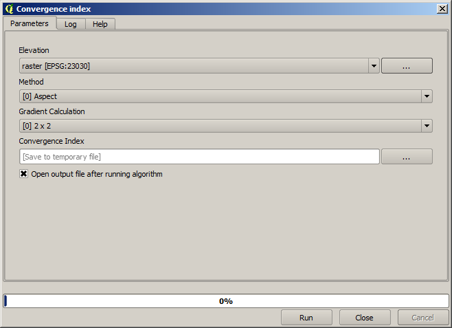
Parameters Dialog
This dialog is used to set the input values that the algorithm needs to be executed. It shows a table where input values and configuration parameters are to be set. It of course has a different content, depending on the requirements of the algorithm to be executed, and is created automatically based on those requirements. On the left side, the name of the parameter is shown. On the right side, the value of the parameter can be set.
Les algorithmes différeront par le nombre et le type de paramètres, mais la structure sera la même pour tous. Les paramètres présents dans la table pourront être un des types suivants.
A raster layer, to select from a list of all such layers available (currently opened) in QGIS. The selector contains as well a button on its right-hand side, to let you select filenames that represent layers currently not loaded in QGIS.
A vector layer, to select from a list of all vector layers available in QGIS. Layers not loaded in QGIS can be selected as well, as in the case of raster layers, but only if the algorithm does not require a table field selected from the attributes table of the layer. In that case, only opened layers can be selected, since they need to be open so as to retrieve the list of field names available.
Vous verrez un bouton pour chaque sélecteur de couche de vecteur, comme le montre la figure ci-dessous.
Figure Processing 8:
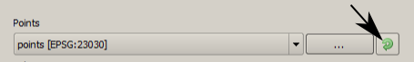
Vector iterator button
Si l’algorithme propose plusieurs boutons d’itération, vous ne pourrez en activer qu’un seul. Si un bouton correspondant à une couche vecteur est activé, l’algorithme s’exécutera successivement sur chacune des entités de la couche plutôt que sur la couche en entier, produisant alors autant de sorties que de nombre d’exécution de l’algorithme. Cela permet d’automatiser un traitement qui doit être réalisé sur chaque entité d’une couche séparément.
- A table, to select from a list of all available in QGIS. Non-spatial
tables are loaded into QGIS like vector layers, and in fact they are treated as
such by the program. Currently, the list of available tables that you will see
when executing an algorithm that needs one of them is restricted to
tables coming from files in dBase (
.dbf) or Comma-Separated Values (.csv) formats. Une option, à choisir dans une liste d’options possibles.
- A numerical value, to be introduced in a text box. You will find a button by its side. Clicking on it, you will see a dialog that allows you to enter a mathematical expression, so you can use it as a handy calculator. Some useful variables related to data loaded into QGIS can be added to your expression, so you can select a value derived from any of these variables, such as the cell size of a layer or the northernmost coordinate of another one.
Figure Processing 9:
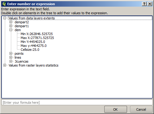
Number Selector
Un intervalle, où doivent être remplies les valeurs minimales et maximales.
Une chaîne de texte, à mettre dans le champ correspondant.
Le num d’un champ, à choisir dans la liste des attributs d’une couche vectorielle ou d’une table préalablement sélectionnées.
Un système de coordonnées de référence. Vous pouvez saisir le code EPSG directement dans la zone de texte ou le sélectionner depuis la fenêtre de sélection du SCR qui apparaît lorsque vous cliquez sur le bouton à droite
Une emprise, à entrer sous la forme des quatre limites
xmin,xmax,ymin,ymax. En cliquant sur le bouton situé à droite du sélecteur, un menu apparaîtra, vous permettant de choisir l’emprise courante du canevas ou de le sélectionner avec la souris sur le canevas.Figure Processing 10

Extent selector
Dans le premier cas s’affichera une fenêtre comme celle-ci.
Figure Processing 11

Extent List
Dans le second cas, la fenêtre de paramètres sera cachée afin de vous permettre de cliquer et glisser sur le canevas. Une fois le rectangle délimité, la fenêtre réapparaîtra, contenant les valeurs de l’emprise choisie.
Figure Processing 12:
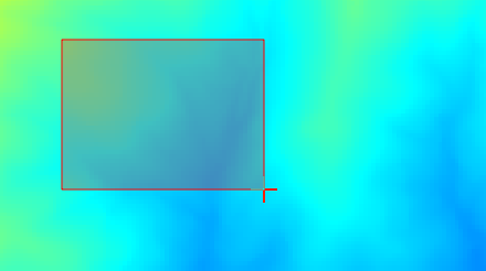
Extent Drag
A list of elements (whether raster layers, vector layers or tables), to select from the list of such layers available in QGIS. To make the selection, click on the small button on the left side of the corresponding row to see a dialog like the following one.
Figure Processing 13:
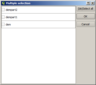
Multiple Selection
Une petite table, à éditer par l’utilisateur, pour définir certains paramètres tels que tables de recherche ou le produit de convolution.
Cliquez sur le bouton sur le côté droit pour voir la table et éditer ses valeurs.
Figure Processing 14:
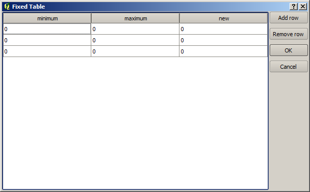
Fixed Table
Selon l’algorithme, les lignes sont modifiables ou non, en utilisant les boutons situés à droite de la fenêtre.
You will find a [Help] tab in the the parameters dialog. If a help file is available, it will be shown, giving you more information about the algorithm and detailed descriptions of what each parameter does. Unfortunately, most algorithms lack good documentation, but if you feel like contributing to the project, this would be a good place to start.
A propos des projections
Algorithms run from the processing framework — this is also true of most of the external applications whose algorithms are exposed through it. Do not perform any reprojection on input layers and assume that all of them are already in a common coordinate system and ready to be analized. Whenever you use more than one layer as input to an algorithm, whether vector or raster, it is up to you to make sure that they are all in the same coordinate system.
Note that, due to QGIS‘s on-the-fly reprojecting capabilities, although two layers might seem to overlap and match, that might not be true if their original coordinates are used without reprojecting them onto a common coordinate system. That reprojection should be done manually, and then the resulting files should be used as input to the algorithm. Also, note that the reprojection process can be performed with the algorithms that are available in the processing framework itself.
By default, the parameters dialog will show a description of the CRS of each layer along with its name, making it easy to select layers that share the same CRS to be used as input layers. If you do not want to see this additional information, you can disable this functionality in the processing configuration dialog, unchecking the Show CRS option.
Si vous essayez d’exécuter un algorithme avec deux ou plusieurs couches en entrée avec des SCR non identiques, une fenêtre d’alerte s’affichera.
Vous pourrez toujours exécuter l’algorithme mais sachez que dans la plupart des cas, ceci générera des résultats erronés, comme des couches vides du fait de couches en entrée qui ne se superposent pas.
Les données générées par les algorithmes
Les données générées par un algorithme peuvent être des types suivants :
Une couche raster
Une couche vectorielle
Une table
Un fichier HTML (utilisé pour les sorties texte et graphiques)
These are all saved to disk, and the parameters table will contain a text box corresponding to each one of these outputs, where you can type the output channel to use for saving it. An output channel contains the information needed to save the resulting object somewhere. In the most usual case, you will save it to a file, but the architecture allows for any other way of storing it. For instance, a vector layer can be stored in a database or even uploaded to a remote server using a WFS-T service. Although solutions like these are not yet implemented, the processing framework is prepared to handle them, and we expect to add new kinds of output channels in a near feature.
To select an output channel, just click on the button on the right side of the text box. That will open a save file dialog, where you can select the desired file path. Supported file extensions are shown in the file format selector of the dialog, depending on the kind of output and the algorithm.
The format of the output is defined by the filename extension. The supported
formats depend on what is supported by the algorithm itself. To select a format,
just select the corresponding file extension (or add it, if you are directly typing
the file path instead). If the extension of the file path you entered does not
match any of the supported formats, a default extension (usually .dbf` for
tables, .tif for raster layers and .shp for vector layers) will be
appended to the file path, and the file format corresponding to that extension will
be used to save the layer or table.
If you do not enter any filename, the result will be saved as a temporary file in the corresponding default file format, and it will be deleted once you exit QGIS (take care with that, in case you save your project and it contains temporary layers).
You can set a default folder for output data objects. Go to the configuration
dialog (you can open it from the Processing menu), and in the
General group, you will find a parameter named Output folder.
This output folder is used as the default path in case you type just a filename
with no path (i.e., myfile.shp) when executing an algorithm.
Lorsque vous lancez un algorithme qui utilise une couche vectorielle en mode itératif, le chemin de fichier entré est pris comme chemin de base pour tous les fichiers de sortie, dont le nom correspondra au nom du fichier de base suivi du numéro d’index d’itération. L’extension du fichier (et le format) sera la même pour tous les fichiers générés.
Apart from raster layers and tables, algorithms also generate graphics and text as HTML files. These results are shown at the end of the algorithm execution in a new dialog. This dialog will keep the results produced by any algorithm during the current session, and can be shown at any time by selecting Processing ‣ Results viewer from the QGIS main menu.
Some external applications might have files (with no particular extension restrictions) as output, but they do not belong to any of the categories above. Those output files will not be processed by QGIS (opened or included into the current QGIS project), since most of the time they correspond to file formats or elements not supported by QGIS. This is, for instance, the case with LAS files used for LiDAR data. The files get created, but you won’t see anything new in your QGIS working session.
Pour les autres types de résultat, vous pourrez choisir de les charger ou non à l’issue de l’exécution de l’algorithme en cochant la case. Par défaut, tous les fichiers sont chargés.
Optional outputs are not supported. That is, all outputs are created. However, you can uncheck the corresponding checkbox if you are not interested in a given output, which essentially makes it behave like an optional output (in other words, the layer is created anyway, but if you leave the text box empty, it will be saved to a temporary file and deleted once you exit QGIS).
Configurer le Module de Traitements
Comme mentionné précédemment, le menu de configuration permet d’accéder à une nouvelle fenêtre dans laquelle vous pouvez paramétrer le fonctionnement des algorithmes. Les paramètres sont regroupés en blocs sélectionnables sur la partie gauche.
Along with the aforementioned Output folder entry, the General block contains parameters for setting the default rendering style for output layers (that is, layers generated by using algorithms from any of the framework GUI components). Just create the style you want using QGIS, save it to a file, and then enter the path to that file in the settings so the algorithms can use it. Whenever a layer is loaded by SEXTANTE and added to the QGIS canvas, it will be rendered with that style.
Le rendu des styles peut être configuré pour chaque algorithme et pour chacune de ses sorties. Cliquez avec le bouton droit sur le nom de l’algorithme dans la boîte à outils et sélectionnez Éditer les styles de rendu. Une fenêtre comme celle-ci apparaitra.
Figure Processing 15:
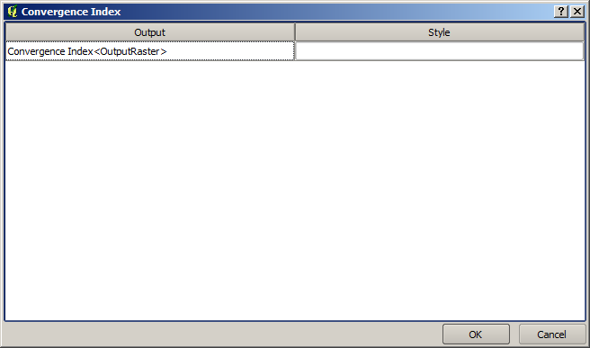
Rendering Styles
Sélectionnez le fichier de style (.qml) que vous souhaitez appliquer à chaque résultat et appuyez sur [OK].
Les autres paramètres de configuration du groupe Général sont les suivants :
Utiliser le nom de fichier comme nom de couche. Le nom de chaque couche créée par un algorithme est défini par l’algorithme lui-même. Dans certains cas, un nom fixe peut être utilisé, ce qui signifie que le même nom sera utilisé, quelle que soit la couche utilisée en entrée. Dans d’autres cas, le nom peut dépendre du nom de la couche d’entrée ou de certains des paramètres utilisés pour exécuter l’algorithme. Si cette case est cochée, le nom sera plutôt issu de celui du fichier de sortie. Notez, que, si la sortie est enregistrée dans un fichier temporaire, le nom de ce fichier temporaire est généralement long et créé de manière à éviter les collisions avec d’autres noms de fichiers déjà existants.
N’utiliser que les entités sélectionnées. Si cette option est sélectionnée, chaque fois qu’une couche vecteur est utilisée comme entrée pour un algorithme, seules ses entités sélectionnées seront utilisées. Si aucune entité de la couche n’est sélectionnée, toutes seront utilisées.
Script Pré-exécution et Script Post-exécution. Ces paramètres font référence à des scripts écrits à l’aide des fonctions du menu Traitements et sont expliqués dans la section abordant les algorithmes et la console.
Vous trouverez également un bloc Général pour chaque fournisseur d’algorithmes. Chaque bloc contient une rubrique Activé pour le faire apparaître dans la boîte à outils. De plus, certains fournisseurs ont leurs propres options de configuration. Cela sera détaillé dans la description de chaque fournisseur.