8.3. Lesson: 지형 분석

래스터가 표현하고 있는 지형에 대해 더 깊이 이해할 수 있게 해주는 특정한 래스터 형식이 있습니다. 수치 표고 모델(DEM)이 이런 점에서 특히 유용합니다. 이 강의에서는 지형 분석을 이용해서, 이전 모듈에서 다뤘던 주거 구역 개발에 대해 더 자세히 알아보도록 하겠습니다.

이 강의의 목표: 지형 분석을 이용해서 지형에 대해 더 많은 정보를 끌어내기.

8.3.1. Follow Along: 음영기복도 계산

We are going to use the same DEM layer as in the previous lesson. If you are starting this chapter from scratch use the Browser panel and load the raster/SRTM/srtm_41_19.tif.

The DEM layer shows you the elevation of the terrain, but it can sometimes seem a little abstract. It contains all the 3D information about the terrain that you need, but it doesn’t look like a 3D object. To get a better look at the terrain, it is possible to calculate a hillshade, which is a raster that maps the terrain using light and shadow to create a 3D-looking image.

We are going to use algorithms of Raster ‣ Raster terrain analysis menu.

1. Click on the Hillshade menu

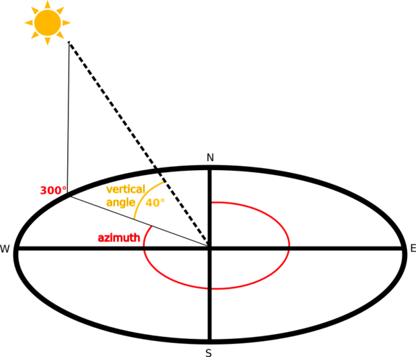
2. The algorithm allows you to specify where the position of the light source: the Azimuth parameter has values from 0 (North) through 90 (East), 180 (South) and 270 (West) while the Vertical angle sets how high the light is. We will leave the default values:

   

3. Save the file in a new folder raster_analysis within the folder exercise_data with the name hillshade

4. Finally click on Run

이제 다음과 같이 hillshade 라는 새 레이어가 생성되었습니다.

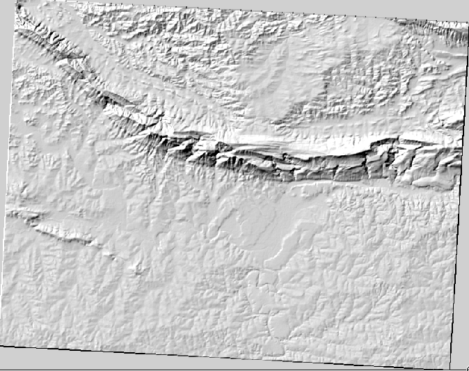
멋진 3D로 보입니다만, 좀 더 향상시킬 수 있을까요? 음영기복도 그 자체로는 마치 석고 모형처럼 보입니다. 다른, 좀 더 다채로운 래스터들과 어떻게 함께 사용할 수는 없을까요? 물론 할 수 있습니다. 음영기복도를 오버레이로서 사용한다면 말이죠.

8.3.2. Follow Along: 음영기복도를 오버레이로 사용

음영기복도는 낮 동안의 특정 시간의 햇빛에 대한 유용한 정보를 제공할 수 있습니다. 하지만 맵을 더 보기 좋게 하기 위한 심미적 목적을 위해서도 사용할 수 있습니다. 이렇게 하려면 음영기복도를 거의 투명하게 설정하면 됩니다.

1. Change the symbology of the original srtm_41_19 layer to use the Pseudocolor scheme as in the previous exercise

2. Hide all the layers except the srtm_41_19 and hillshade layers

3. Click and drag the srtm_41_19 to be beneath the hillshade layer in the Layers panel

4. Set the hillshade layer to be transparent by clicking on the Transparency tab in the layer properties

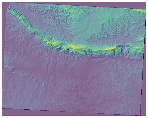
5. Set the Global opacity to 50%.

   You’ll get a result like this:

   

6. Switch the hillshade layer off and back on in the Layers panel to see the difference it makes.

음영기복도를 이런 식으로 사용하면 경관의 지형을 향상시킬 수 있습니다. 만약 그 효과가 미미하다고 느껴진다면, hillshade 레이어의 투명도를 조절할 수 있습니다. 하지만 물론, 음영기복도가 밝아질수록 그 아래의 색상은 침침해질 것입니다. 여러분이 만족할 수 있는 균형을 찾아야 합니다.

Remember to save the project when you are done.

8.3.3. Follow Along: 경사도 계산

지형에 대해 알아두면 좋은 점 가운데 하나는 얼마나 가파르냐는 것입니다. 예를 들어 어떤 토지에 집을 짓고 싶다고 할 때, 그 토지는 어느 정도 평평해야 할 것입니다.

To do this, you need to use the Slope algorithm of the Processing ‣ Raster terrain analysis.

1. Open the algorithm

2. Choose srtm_41_19 as the Elevation layer

3. Save the output as a file with the name slope in the same folder as the hillshade

4. Click on Run

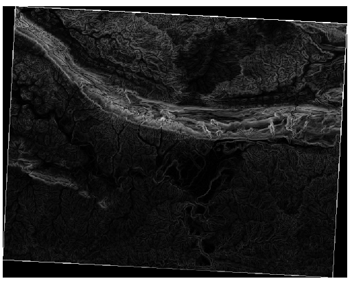
Now you’ll see the slope of the terrain, with black pixels being flat terrain and white pixels, steep terrain:

8.3.4. Try Yourself Calculating the aspect

Aspect is the compass direction that the slope of the terrain faces. An aspect of 0 means that the slope is North-facing, 90 East-facing, 180 South-facing, and 270 West-facing.

Since this study is taking place in the Southern Hemisphere, properties should ideally be built on a north-facing slope so that they can remain in the sunlight.

Use the Aspect algorithm of the Processing ‣ Raster terrain analysis to get the layer.

결과 확인

8.3.5. Follow Along: 래스터 계산기 사용

벡터 분석 강의에서 마지막으로 다뤘던 부동산 중개업자 문제를 다시 떠올려보십시오. 그때의 구매자가 지금은 건물을 산 다음 부지 내에 작은 집을 짓고 싶어 한다고 해봅시다. 남반구에서 이런 개발에 이상적인 계획은 우선 5˚ 미만 경사의 북쪽을 면한 토지가 있어야 할 것입니다. 그러나 경사가 2˚ 미만인 경우, 향은 문제가 되지 않습니다.

다행히 여러분에게는 이미 경사는 물론 향을 보여주는 래스터가 있습니다. 그런데 이 두 가지 조건을 동시에 만족하는 곳을 알 도리가 없죠. 어떻게 이런 분석을 할 수 있을까요?

그 답은 Raster calculator 가 가지고 있습니다.

QGIS has different raster calculators available:

• Raster ‣ Raster Calculator

• Processing ‣ Raster Analysis ‣ Raster calculator

• Processing ‣ GDAL ‣ Raster miscellaneous ‣ Raster calculator

• SAGA ‣ Raster calculus ‣ Raster calculator

Each tool is leading to the same results, but the syntax may be slightly different and the availability of operators may vary.

We will use Processing ‣ Raster Analysis ‣ Raster calculator.

1. Open the tool by double clicking on it.

   • The upper left part of the dialog lists all the raster layers loaded in the legend as name@N where name is the name of the layer and N is the raster band used.

   • In the upper right part you will see a lot of different operators: stop for a moment to think that a raster is an image, you should see it as a 2D matrix filled with numbers.

2. North is at 0 (zero) degrees, so for the terrain to face north, its aspect needs to be greater than 270 degrees and less than 90 degrees. Therefore the formula is:

   aspect@1 <= 90 OR aspect@1 >= 270
   

3. You have now to set up the raster details, like the cell size, extent and CRS. This can be done manually by filling or it can be automatically set by choosing a Reference layer. Choose this last option by clicking on the … button next to the Reference layer(s) parameter.

4. In the dialog, choose the aspect layer because we want to obtain a layer with the same resolution.

5. Save the layer as aspect_north.

   The dialog should look like:

   

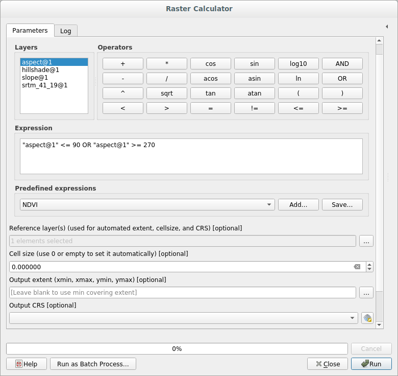
6. Finally click on Run.

결과는 다음과 같을 것입니다.

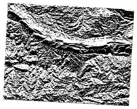
The output values are 0 or 1. What does it mean? The formula we wrote contains the conditional operator OR: therefore the final result will be False (0) and True (1).

8.3.6. Try Yourself More slopes

이제 향 작업을 끝냈으니, DEM 레이어에 대한 두 가지 새로운 분석을 생성해봅시다.

• The first will be to identify all areas where the slope is less than or equal to 2 degrees.

• The second is similar, but the slope should be less than or equal to 5 degrees.

• Save them under exercise_data/raster_analysis as slope_lte2.tif and slope_lte5.tif.

결과 확인

8.3.7. Follow Along: 래스터 분석 결과 결합

이제 다음과 같은 DEM 레이어의 세 가지 분석 래스터가 생겼습니다.

• aspect_north : 북쪽을 면한 지형

• slope_lte2: 경사가 2˚ 이하인 지형

• slope_lte5: 경사가 5˚ 이하인 지형

Where the conditions of these layers are met, they are equal to 1. Elsewhere, they are equal to 0. Therefore, if you multiply one of these rasters by another one, you will get the areas where both of them are equal to 1.

만족해야 하는 조건은 다음과 같습니다. 경사가 5˚ 이하이며, 북쪽을 면하는 지형일 것, 다만 경사가 2˚ 이하인 곳은 해당 지형이 어느쪽을 면하든지 상관 없슴.

Therefore, you need to find areas where the slope is at or below 5 degrees AND the terrain is facing north, OR the slope is at or below 2 degrees. Such terrain would be suitable for development.

이 기준들을 만족하는 지역을 계산하려면,

1. Open your Raster calculator again

2. Use the Layer panel, the Operators buttons, and your keyboard to build this expression in the Expressions text area:

   ( aspect_north@1 = 1 AND slope_lte5@1 = 1 ) OR slope_lte2@1 = 1
   

3. Set the Reference layer(s) parameter as the aspect_north (it does not matter if you choose another one given that all the layers have been calculated from srtm_41_19)

4. Save the output under exercise_data/raster_analysis/ as all_conditions.tif

5. Click Run

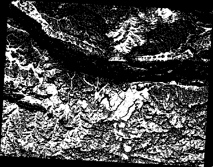
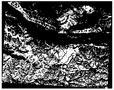
Your results:

8.3.8. Follow Along: 래스터 단순화

앞의 이미지에서 볼 수 있듯이, 이렇게 결합된 분석의 결과물은 조건을 만족하는 수많은, 아주 작은 지역들로 이루어져 있습니다. 그러나 이 결과는 우리의 분석에 그다지 쓸모가 없습니다. 뭔가를 짓기에는 너무 작은 토지들이니까요. 이 쓸모 없는 작은 토지들을 제거해보겠습니다.

1. Open the Sieve tool Processing ‣ GDAL ‣ Raster Analysis

2. Set the Input file to all_conditions, and the Sieved to all_conditions_sieve.tif (under exercise_data/raster_analysis/).

3. Set both the Threshold to 8 and check Use 8-connectedness.

   

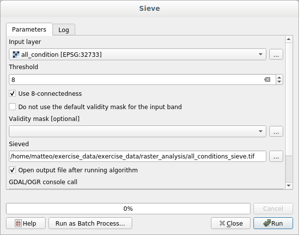
   Once processing is done, the new layer will load into the canvas.

   

   무엇 때문일까요? 그 답은 이 새 래스터 파일의 메타데이터에 있습니다.

4. View the metadata under the Information tab of the Layer Properties dialog. Look the STATISTICS_MINIMUM value: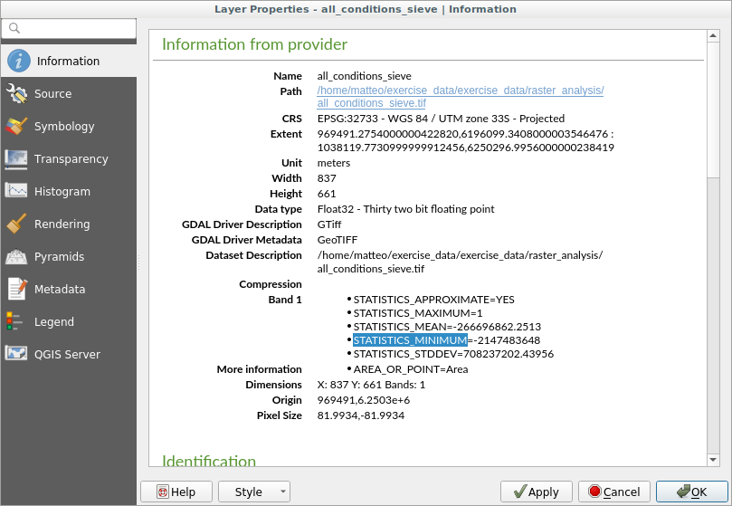

   

   Whereas this raster, like the one it’s derived from, should only feature the values 1 and 0 while it has also a very large negative number. Investigation of the data shows that this number acts as a null value. Since we’re only after areas that weren’t filtered out, let’s set these null values to zero.

5. Open the Raster Calculator again, and build this expression:

   (all_conditions_sieve@1 <= 0) = 0
   

   This will maintain all existing zero values, while also setting the negative numbers to zero; which will leave all the areas with value 1 intact.

6. Save the output under exercise_data/raster_analysis/ as all_conditions_simple.tif.

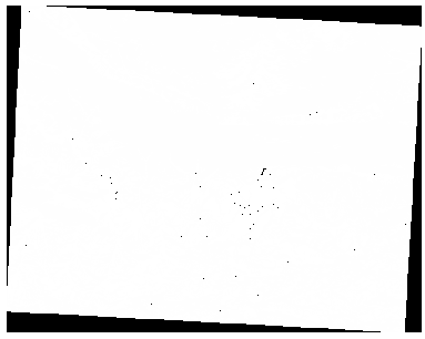
산출물은 다음과 같습니다.

우리가 기대한 산출물입니다. 이전 결과물을 단순화시킨 버전이죠. 어떤 도구의 결과물이 기대했던 것과 다를 경우, 문제를 해결 하는 데 메타데이터(및, 적용 가능할 경우 벡터 속성)을 살펴보는 작업이 필수적일 수도 있습니다.

8.3.9. Follow Along: Reclassifying the Raster

We use the Raster calculator tool to make some calculation on raster layer. There is another powerful tool that we can use to better extract information from existing layers.

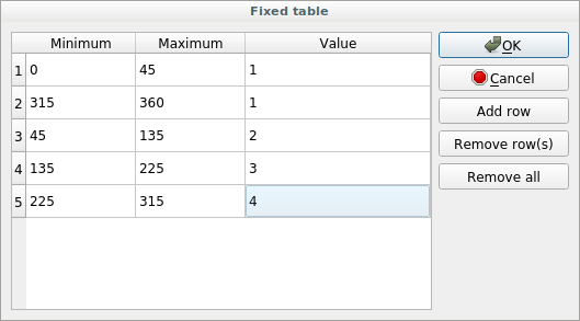
Back to the aspect layer: we know now that it has numeric values within a range from 0 through 360. What we want to do is to reclassify this layer with other discrete values (from 1 to 4) depending on the aspect:

• 1 = North (from 0 to 45 and from 315 to 360);

• 2 = East (from 45 to 135)

• 3 = South (from 135 to 225)

• 4 = West (from 225 to 315)

This operation could be achieved with the raster calculator but the formula would become very very large.

The alternative tool is the Reclassify by table tool within Processing ‣ Raster analysis.

1. Open the tool

2. Choose aspect as the Input raster layer

3. Click on the … of the Reclassification table parameter. A table like dialog will pop up where you can choose the minimum, maximum and new values for each class.

4. Click on the Add row button and add 5 rows. Fill each row as the following picture and click OK:

   

   The method used by the algorithm to treat the threshold values of each class is defined by the Range boundaries parameter.

5. Save the layer as reclassified in the exercise_data/raster_analysis/ folder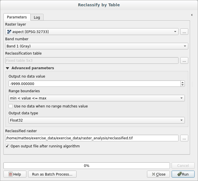

   

6. Click on Run

If you compare the native aspect layer with the reclassified one, there are not big differences. But giving a look at the legend you can see that the values go from 1 to 4.

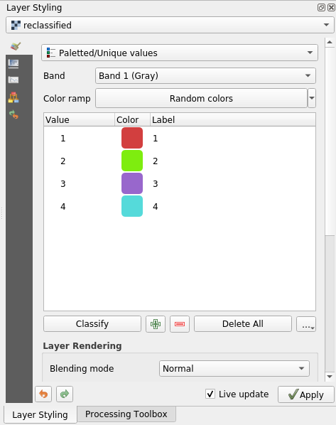
Let’s give this layer a better style.

1. Open the Layer Styling panel

2. Choose Paletted/Unique values instead of Singleband gray

3. Click on the Classify button to automatically fetch the values and assign them random colors:

   

The output should look like this (you can have different colors given that they have been randomly generated):

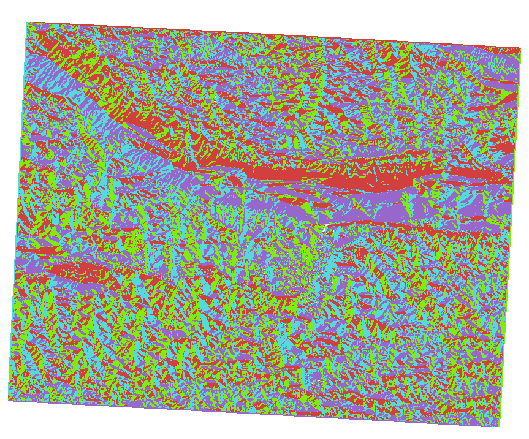
With this reclassification and the paletted style applied to the layer you can immediately see the aspect areas. Cool isn’t it?!

8.3.10. Follow Along: Querying the raster

Unlike vectors, raster layers don’t have an attribute table: each pixel contains one or more numerical values, depending if the raster is singleband or multiband.

All the raster layers we used in this exercise are made by just a single band: depending on the layer, pixel numbers will represent elevation, aspect or slope values.

How can we query the raster layer to know the value of a single pixel? We can use the button to extract this information.

1. Select the tool from the upper toolbar

2. Click on a random location of the srtm_41_19 layer. The Identify Results will appear with the value of the band at the clicked location:

   

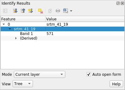
3. You can change the output of the Identify Results panel from the current tree mode to a table one by selecting Table in the View menu at the bottom of the panel: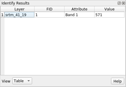

   

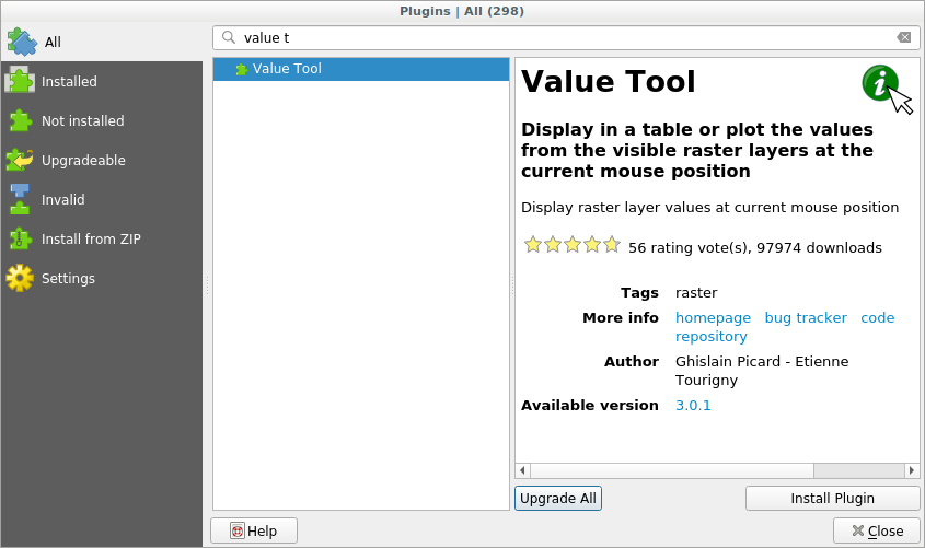
Clicking each pixel to get the value of the raster could become annoying after a while. We can use the Value Tool plugin to solve this problem.

1. Go to Plugins ‣ Manage/Install Plugins…

2. In the All tab, type Value Tool in the search box

3. Select the Value Tool plugin, press Install Plugin and then Close the dialog.

   

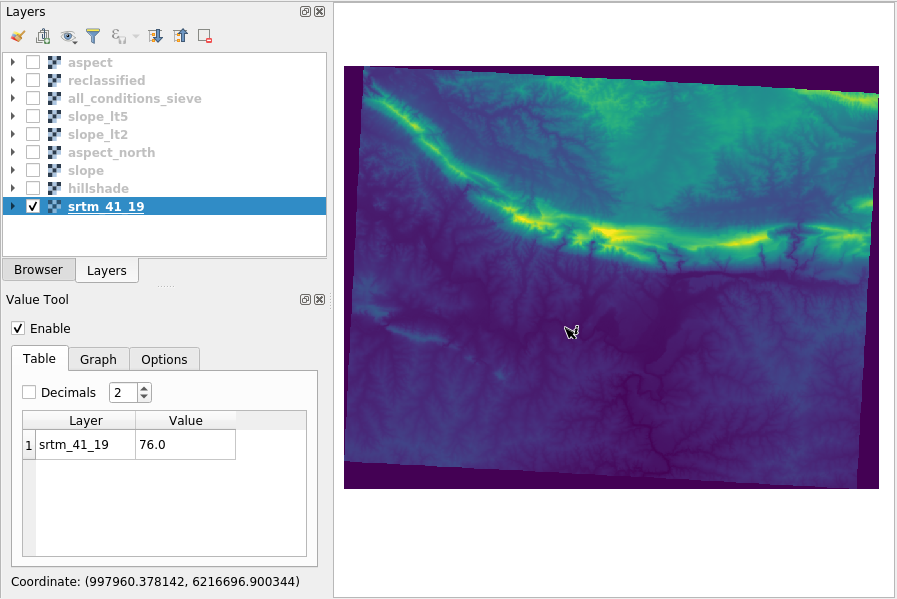
   The new Value Tool panel will appear.

   팁

   If you close the panel you can reopen it by enabling it in the View ‣ Panels ‣ Value Tool or by clicking on the new icon of the toolbar.

4. To use the plugin just check the Enable checkbox and be sure that the srtm_41_19 layer is active (checked) in the Layers panel.

5. Move the cursor on the map to immediately know the value of the pixel

   

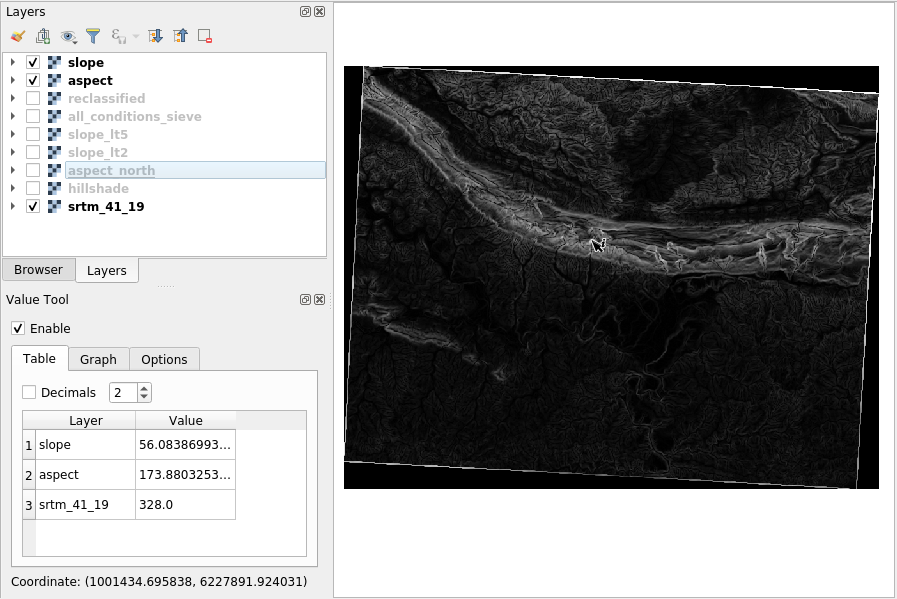
6. But there is more. The Value Tool plugin allows to query all the active raster layers in the Layers panel. Set the aspect and slope layers active again and hover the mouse on the map:

   

8.3.11. In Conclusion

You’ve seen how to derive all kinds of analysis products from a DEM. These include hillshade, slope and aspect calculations. You’ve also seen how to use the raster calculator to further analyze and combine these results. Finally you learned how to reclassify a layer and how to query the results.

8.3.12. What’s Next?

이제 여러분은 두 가지 분석을 할 수 있습니다. 벡터 분석은 잠재적으로 적합한 계획을 보여주며, 래스터 분석은 잠재적으로 적합한 지형을 보여줍니다. 이들을 어떻게 결합해야 문제에 대한 최종 결론을 얻을 수 있을까요? 이것이 다음 모듈에서 시작하는 강의의 주제입니다.