18. Answer Sheet
18.1. Results For Ajout de votre première Couche
18.1.1.  Préparation
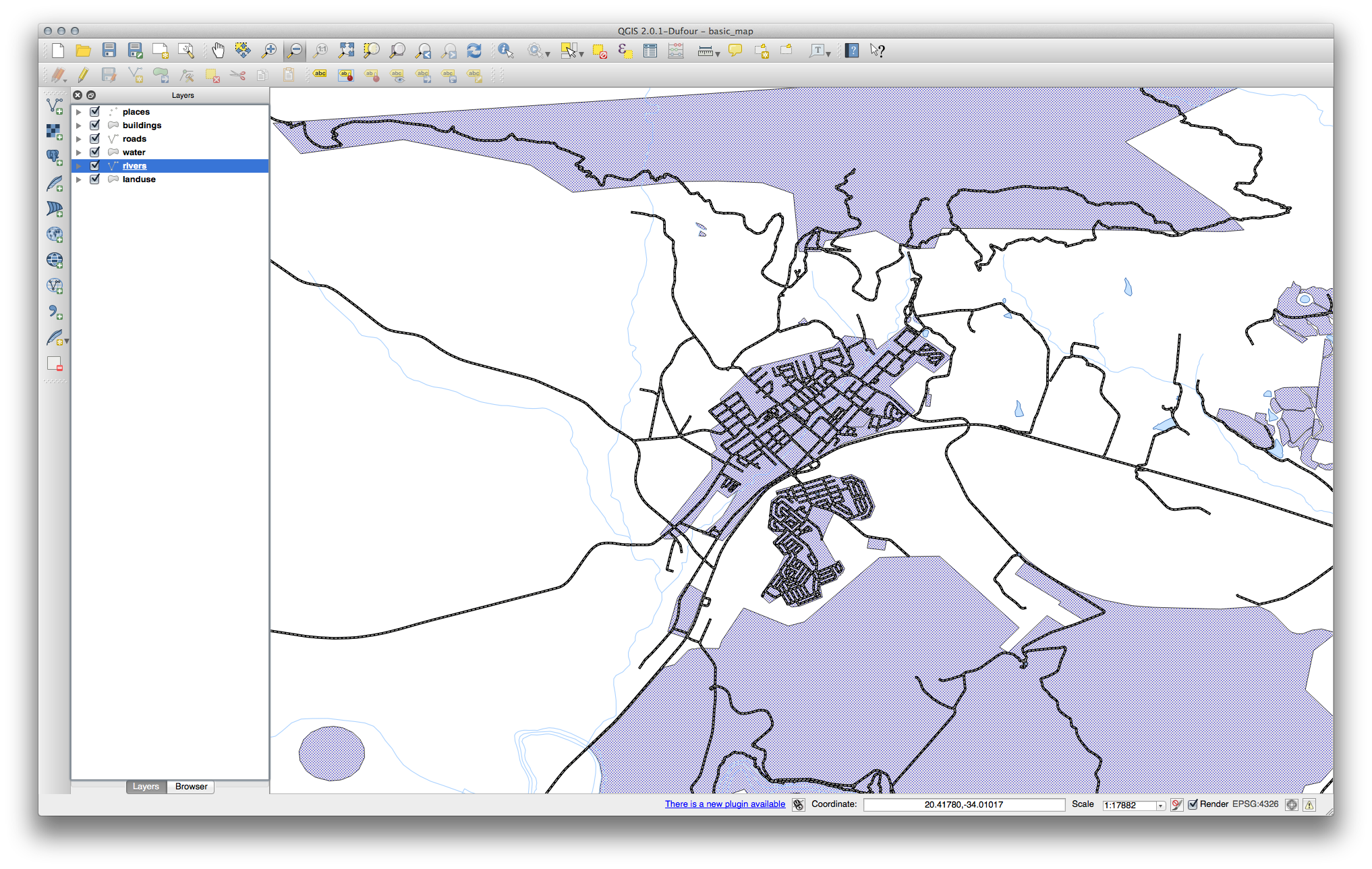
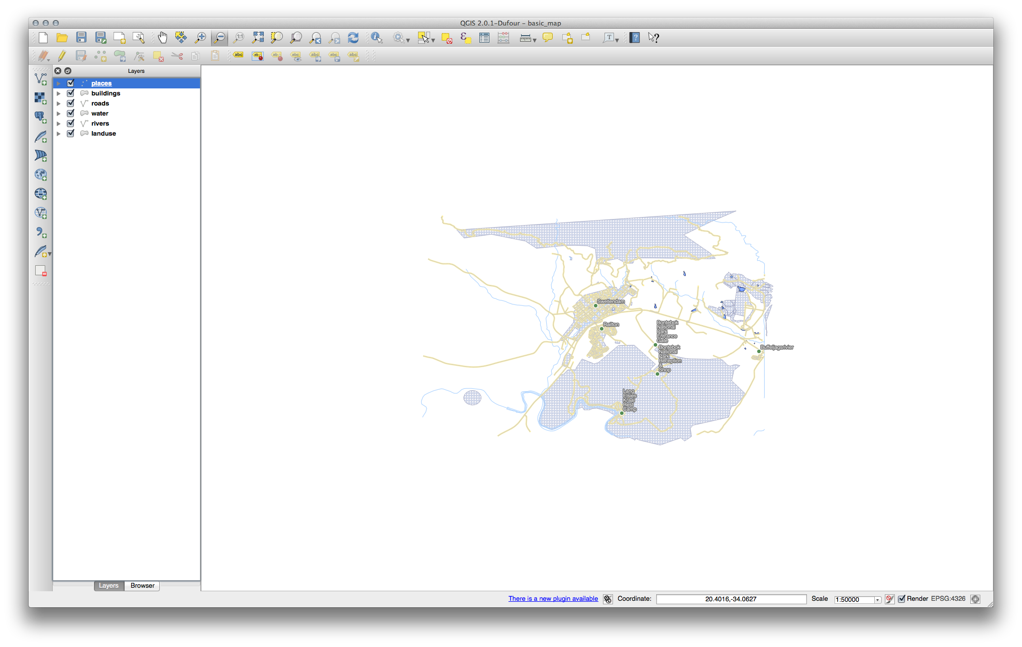
You should see a lot of lines, symbolizing roads. All these lines are in the vector layer that you just loaded to create a basic map.
18.2. Results For Un Aperçu de l’Interface
18.2.1. Aperçu (Partie 1)
Refer back to the image showing the interface layout and check that you remember the names and functions of the screen elements.
18.2.2. Aperçu (Partie 2)
Sauvegarder sous
Zoom sur la couche
Aide
Rendu on/off
Mesurer une longueur
18.3. Results For Travailler avec les Données Vecteurs
18.3.1. Shapefiles
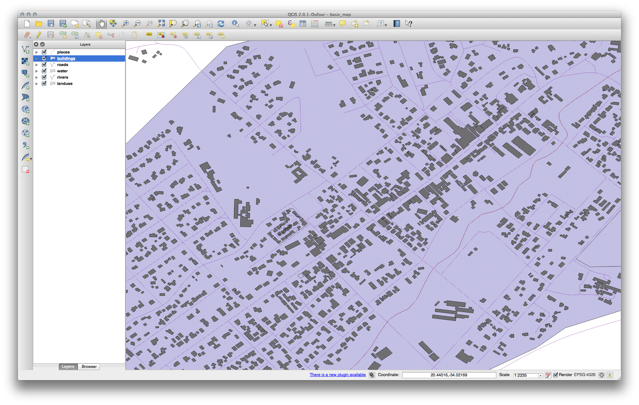
Il devrait y avoir cinq couches sur la carte:
- places
- water
- buildings
rivers et
- roads.
18.3.2. Bases de Données
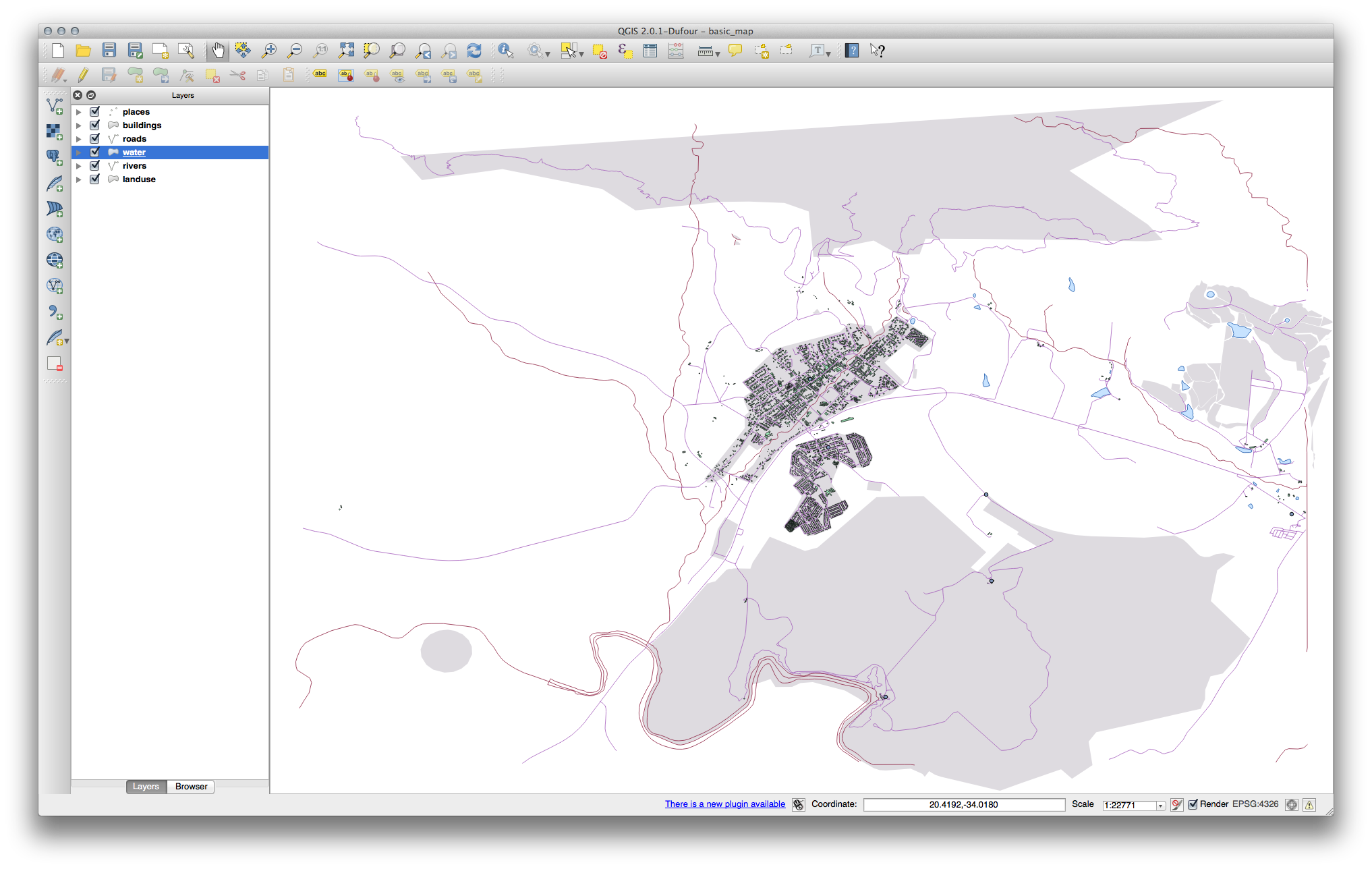
All the vector layers should be loaded into the map. It probably won’t look nice yet though (we’ll fix the ugly colors later).
18.4. Results For Style
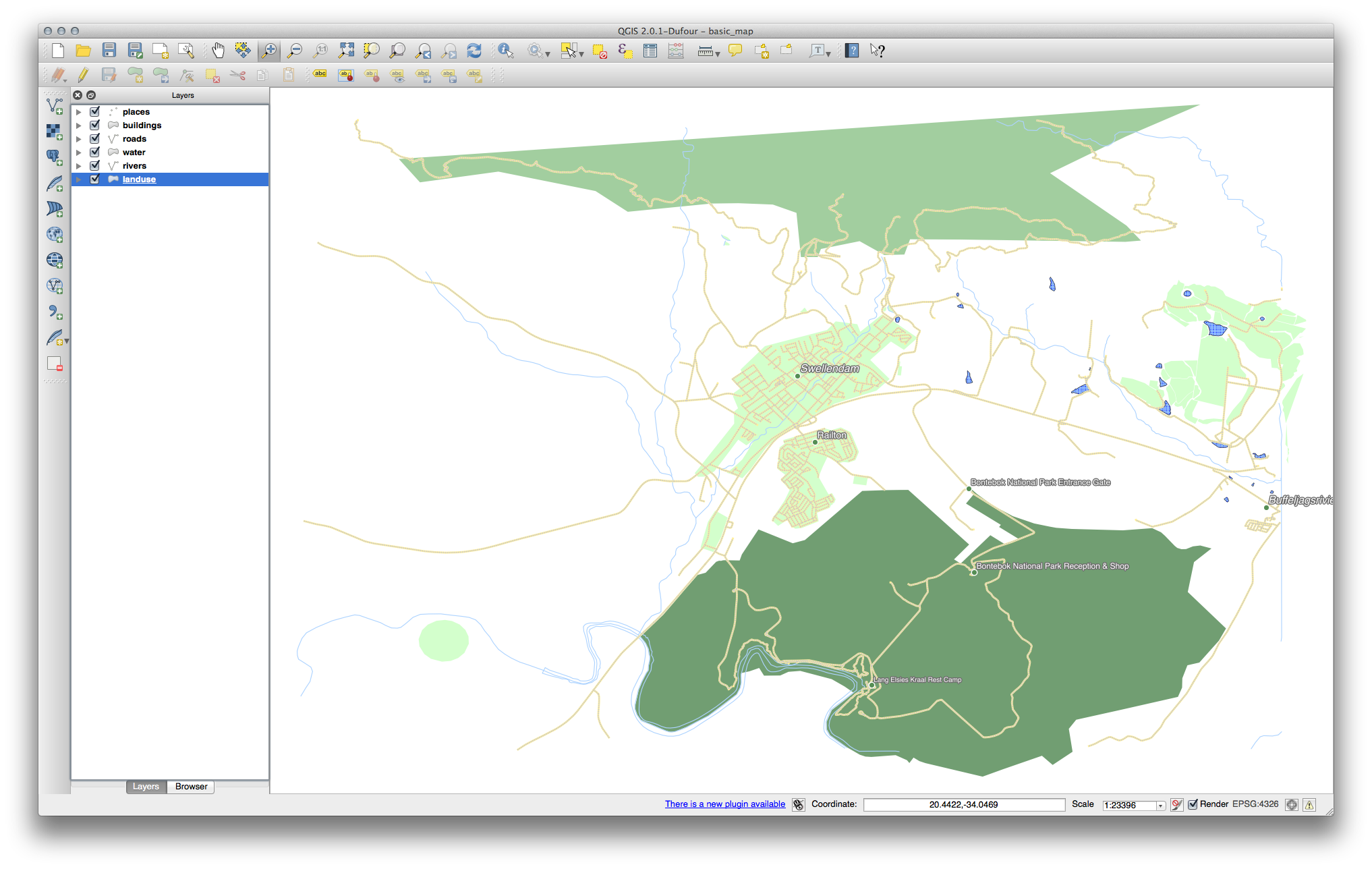
18.4.1. Couleurs
Vérifiez que les couleurs changent telles que vous l’escomptez.
Il suffit de changer la couche water pour l’instant. Un exemple est indiqué ci-après, mais il pourrait être différent de ce que vous avez selon la couleur que vous avez choisie.
Note
Si vous souhaitez travailler sur une seule couche à la fois et ne pas être perturbé par d’autres couches, vous pouvez cacher le contenu de ces couches en cliquant sur la case à cocher à côté du nom dans la liste des couches. Si la case est vide, alors la couche ne sera pas affichée.
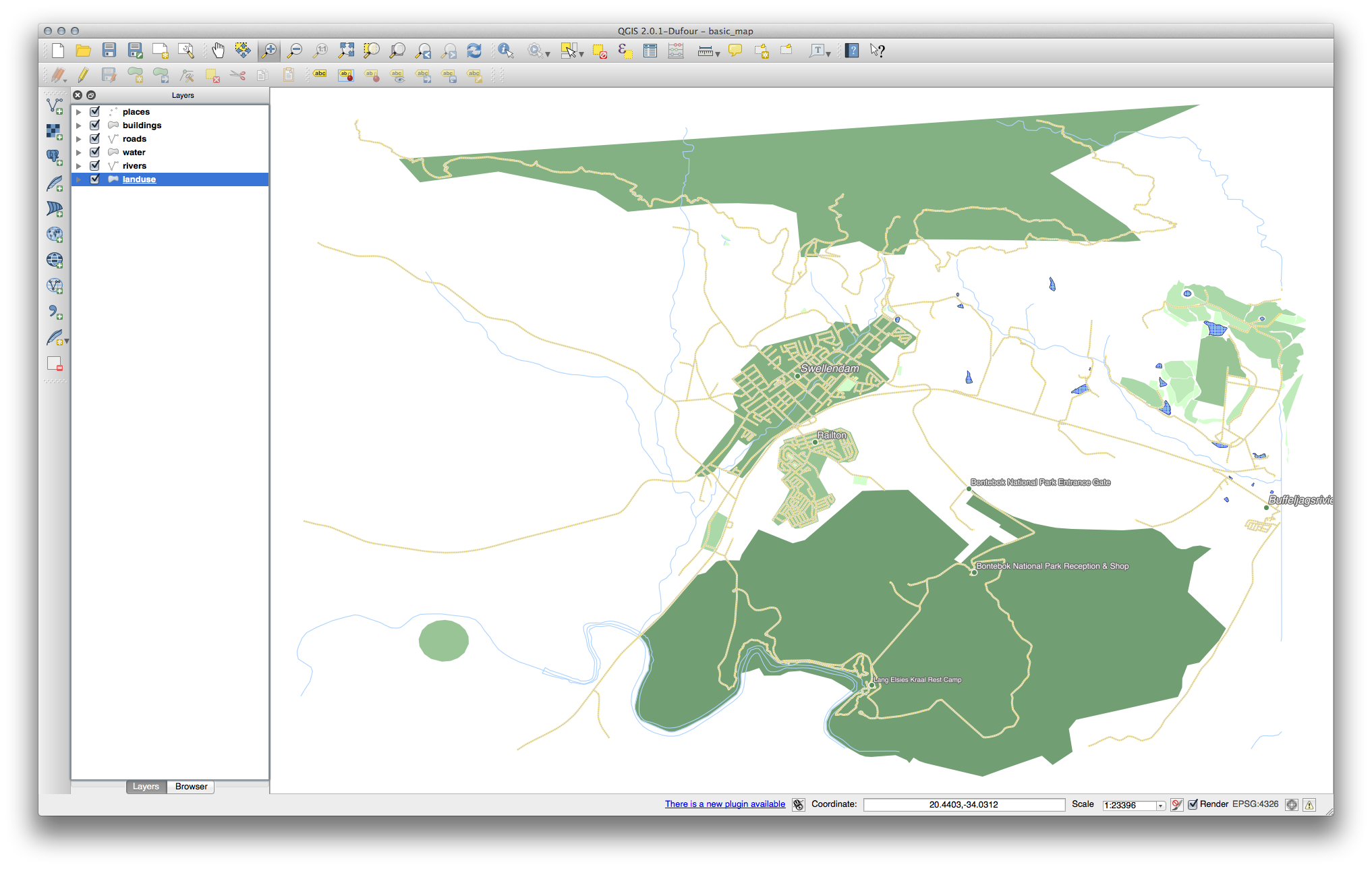
18.4.2. Symbol Structure
Votre carte devrait maintenant ressembler à ça:
Si vous êtes un utilisateur débutant, vous pouvez vous arrêter ici.
Utilisez la méthode ci-dessus pour modifier les couleurs et les styles pour toutes les couches restantes.
Essayez d’utiliser des couleurs naturelles selon les objets. Par exemple, une route ne devrait pas être rouge ou bleue, mais peut être en gris ou en noir.
De même, n’hésitez pas à expérimenter différents paramètres de Style de remplissage et de Style de bordure pour les polygones.
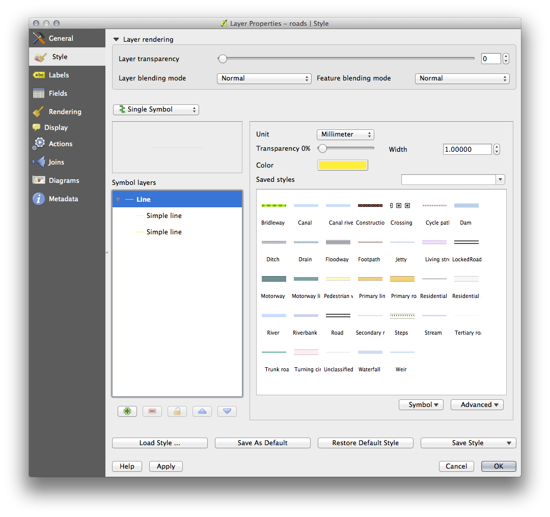
18.4.3.  Symbol Layers
- Customize your buildings layer as you like, but remember that it has to be easy to tell different layers apart on the map.
Voici un exemple:
18.4.4. Niveaux de symboles
To make the required symbol, you need two symbol layers:
The lowest symbol layer is a broad, solid yellow line. On top of it there is a slightly thinner solid gray line.
If your symbol layers resemble the above but you’re not getting the result you want, check that your symbol levels look something like this:
Maintenant, votre carte devrait ressembler à ça:
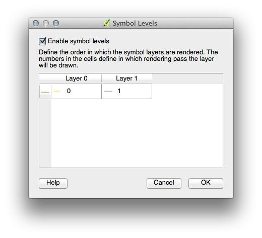
18.4.5.  Symbol Levels
- Adjust your symbol levels to these values:
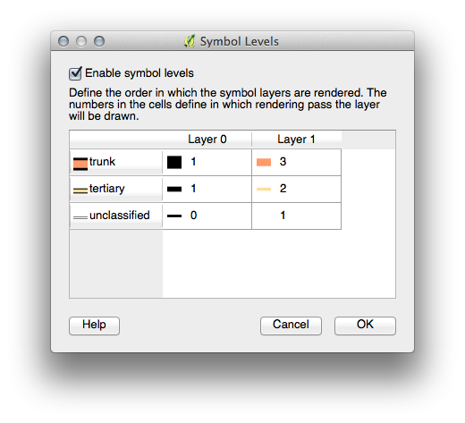
Essayez différentes valeurs afin d’obtenir différents résultats.
Ouvrez à nouveau votre carte originale avant d’aborder l’exercice suivant.
18.5. Results For Données Attributaires
18.5.1. Données Attributaires
Le champ NAME est le plus utile pour afficher les étiquettes. Ceci est dû au fait que toutes ses valeurs sont uniques à chacun des objets et peu susceptibles de contenir la valeur NULL. Si vos données contiennent des valeurs NULL, ne vous inquiétez pas du moment que la plupart de vos places ont des noms.
18.6. Results For L’outil Étiquette
18.6.1. Label Customization (Part 1)
Your map should now show the marker points and the labels should be offset by
2.0 mm: The style of the markers and labels should allow both to be
clearly visible on the map:
18.6.2. Label Customization (Part 2)
Une solution possible aboutit à ce résultat final:
Pour arriver à ce résultat:
Utilisez une Taille de police de
10, une Distance de1,5 mm, une Largeur du symbole et Hauteur du symbole de3.0 mm.En outre, cet exemple utilise l’option Retour à la ligne sur le caractère:
Enter a
spacein this field and click Apply to achieve the same effect. In our case, some of the place names are very long, resulting in names with multiple lines which is not very user friendly. You might find this setting to be more appropriate for your map.
18.6.3. Using Data Defined Settings
Still in edit mode, set the
FONT_SIZEvalues to whatever you prefer. The example uses16for towns,14for suburbs,12for localities and10for hamlets.Pensez à sauvegarder vos modifications et sortir du mode d’édition.
Return to the Text formatting options for the places layer and select
FONT_SIZEin the Attribute field of the font size data override dropdown: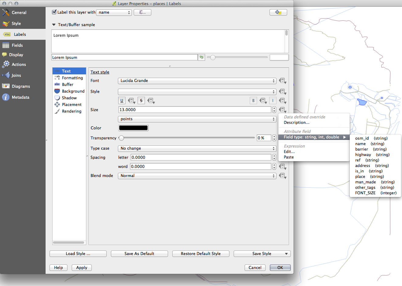
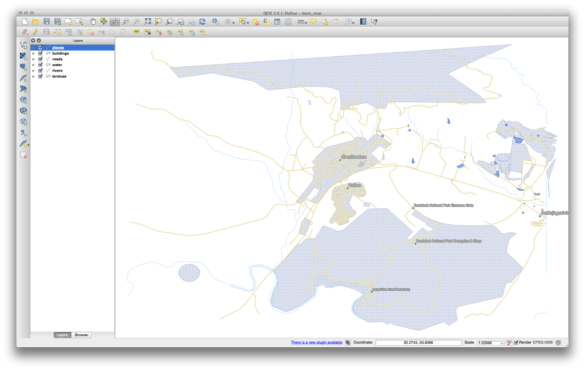
Vos résultats, en utilisant les valeurs ci-dessous, devraient être ceux-ci:
18.7. Results For Classification
18.7.1. Refine the Classification
Utiliser la même méthode que dans le premier exercice de la leçon pour vous débarrasser des bordures:
Les paramètres que vous avez utilisés pourraient ne pas être les mêmes mais, avec Classes = 6 et Mode = Ruptures Naturelles (Jenks) (et bien sûr, en utilisant les mêmes couleurs), la carte ressemblera à ça:
18.8. Results For Creating a New Vector Dataset
18.8.1. Numérisation
Le style importe peu, mais les résultats devraient plus ou moins ressembler à celui-ci:
18.8.2. Topologie: Outil Ajouter un Anneau
La forme exacte importe peu, mais vous devriez obtenir un trou au centre de votre entité, comme sur celle-ci:
Annulez vos modifications avant d’entamer l’exercice du prochain outil.
18.8.3. Topologie: Outil Ajouter une Partie
Tout d’abord, sélectionner Bontebok National Part:
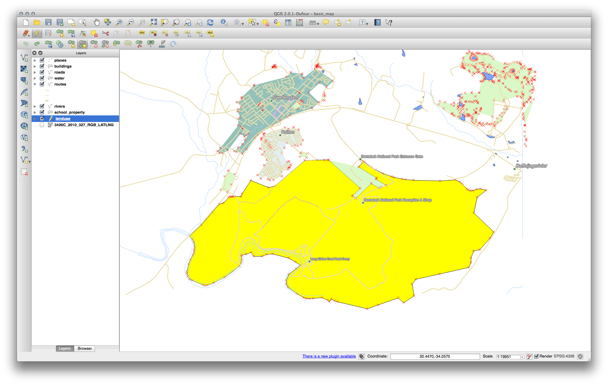
Maintenant, ajoutez votre nouvelle partie:

Annulez vos modifications avant d’entamer l’exercice du prochain outil.
18.8.4. Fusionner les entités
Utilisez l’outil Fusionner les entités sélectionnées en vous assurant d’avoir au préalable sélectionné les deux polygones que vous souhaitez fusionner.
- Use the feature with the OGC_FID of
1as the source of your attributes (click on its entry in the dialog, then click the Take attributes from selected feature button):
Note
- If you’re using a different dataset, it is highly likely that your
- original polygon’s OGC_FID will not be
1. Just choose the feature which has an OGC_FID.
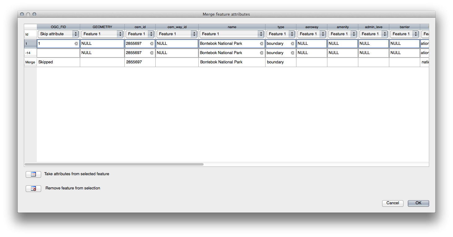
Note
Utiliser l’outil Fusionner les attributs des entités sélectionnées conservera les géométries distinctes mais leur affecte les mêmes attributs.
18.8.5. Formulaires
Pour le TYPE, il y a de toute évidence un nombre maximum de types de voies, et si vous regardez la table attributaire de cette couche, vous verrez qu’ils sont prédéfinis.
Set the widget to Value Map and click Load Data from Layer.
Select roads in the Label dropdown and highway for both the Value and Description options:
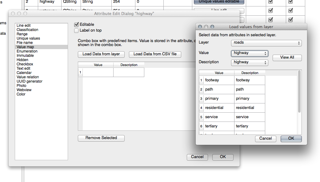
Cliquez sur Ok trois fois.
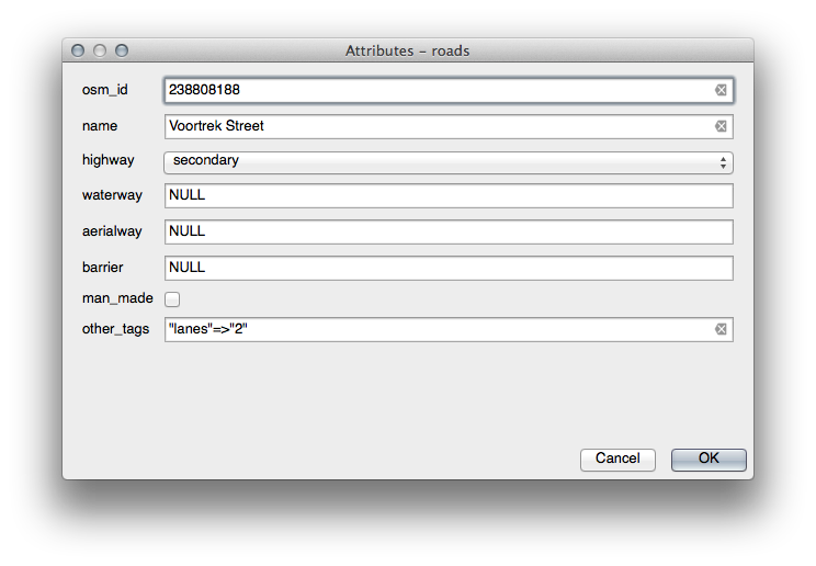
If you use the Identify tool on a street now while edit mode is active, the dialog you get should look like this:
18.9. Results For Analyse vectorielle
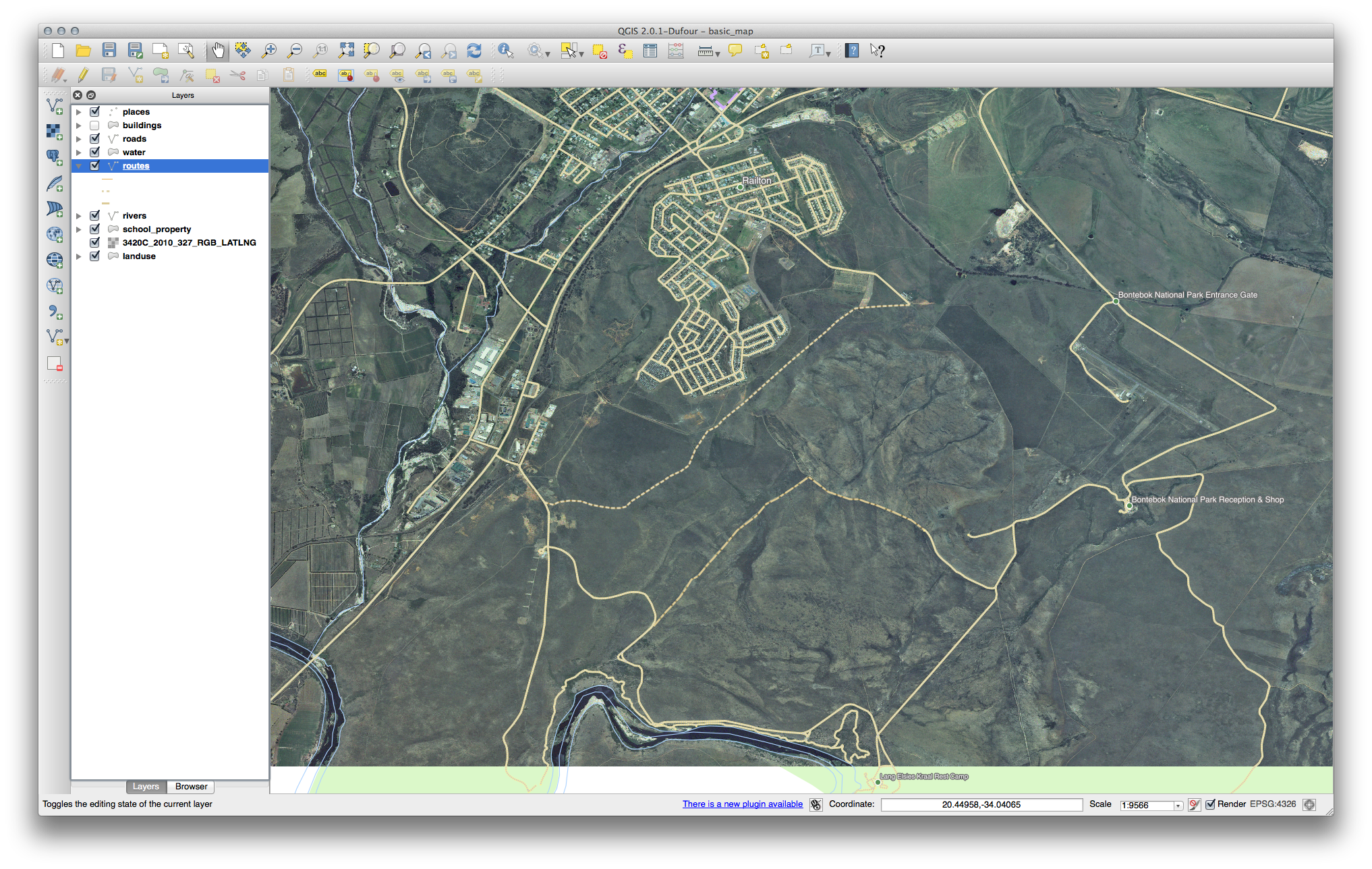
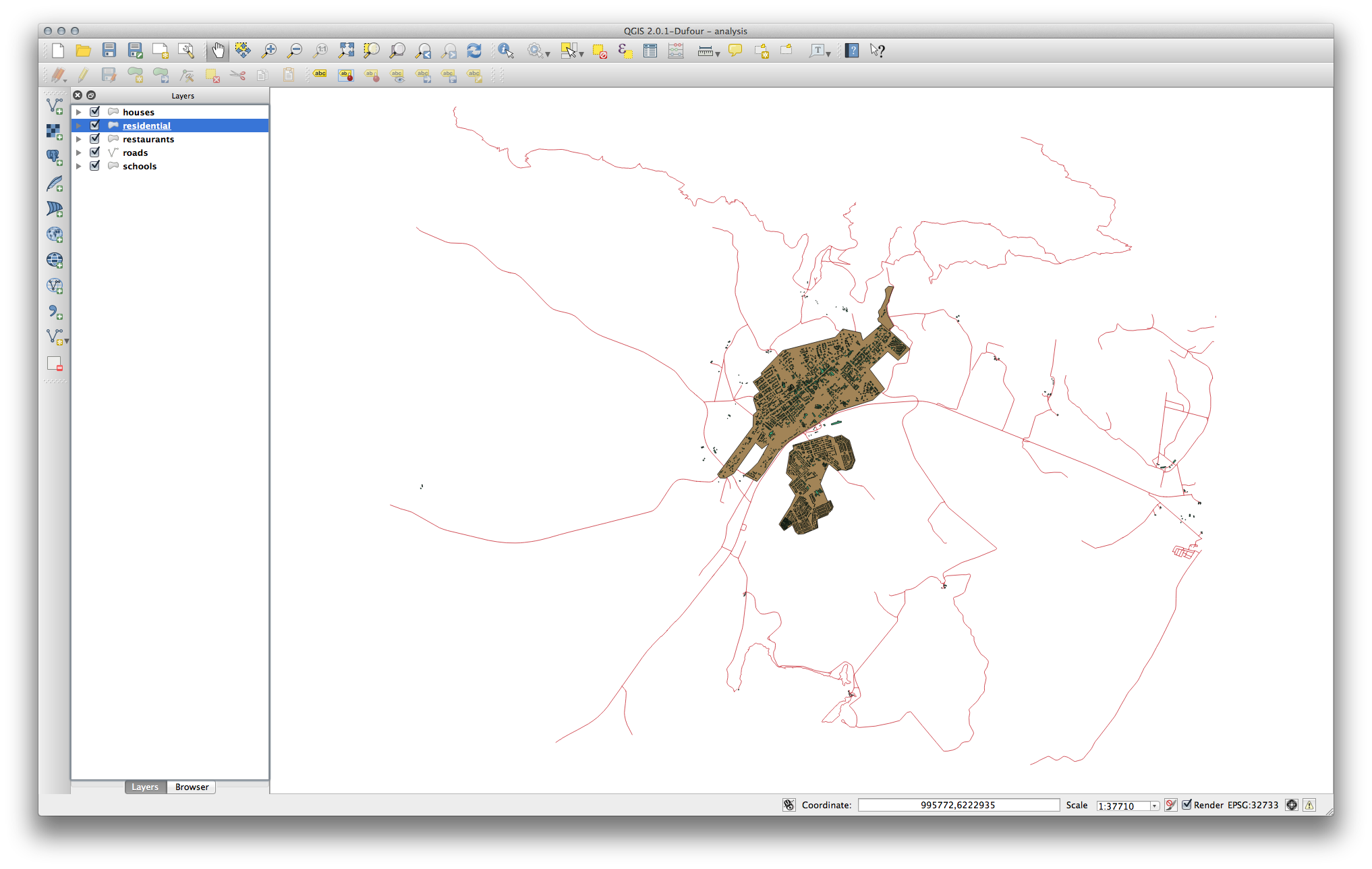
18.9.1. Extraire vos couches à partir des données OSM
For the purpose of this exercise, the OSM layers which we are interested in are
multipolygons and lines. The multipolygons layer contains
the data we need in order to produce the houses, schools and
restaurants layers. The lines layer contains the roads dataset.
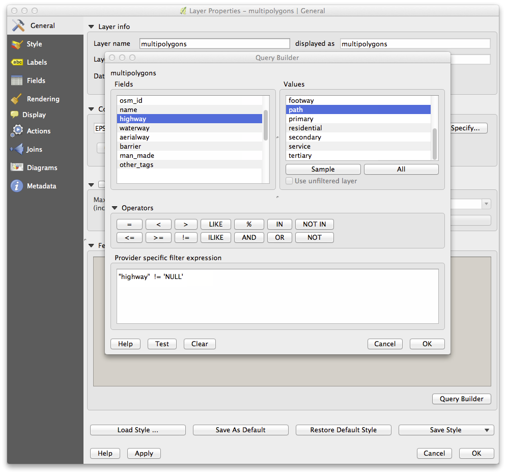
Le Constructeur de requêtes se trouve dans les propriétés de la couche:
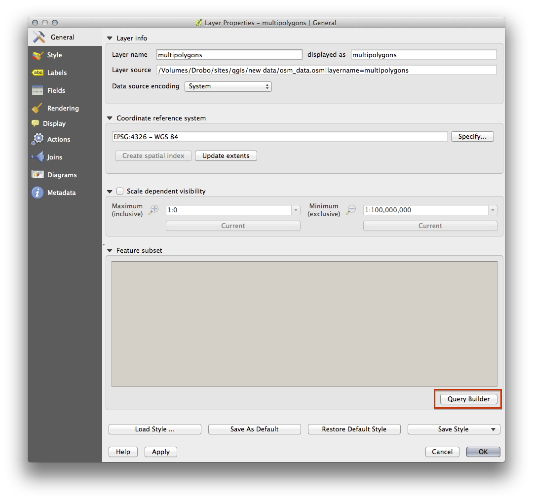
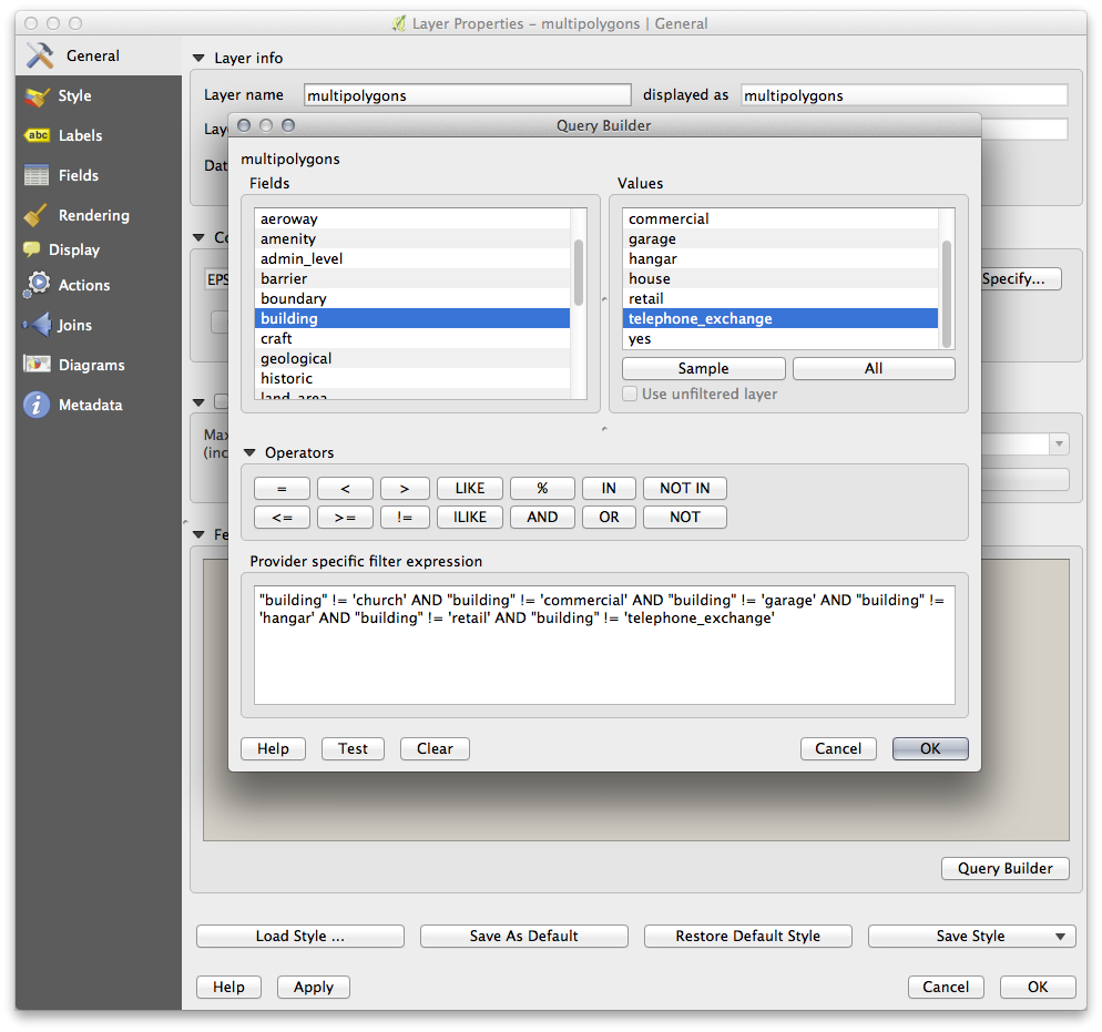
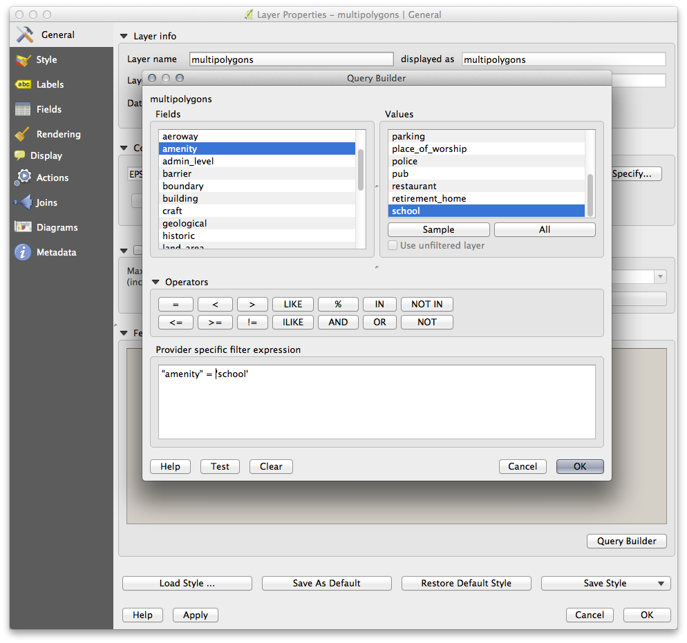
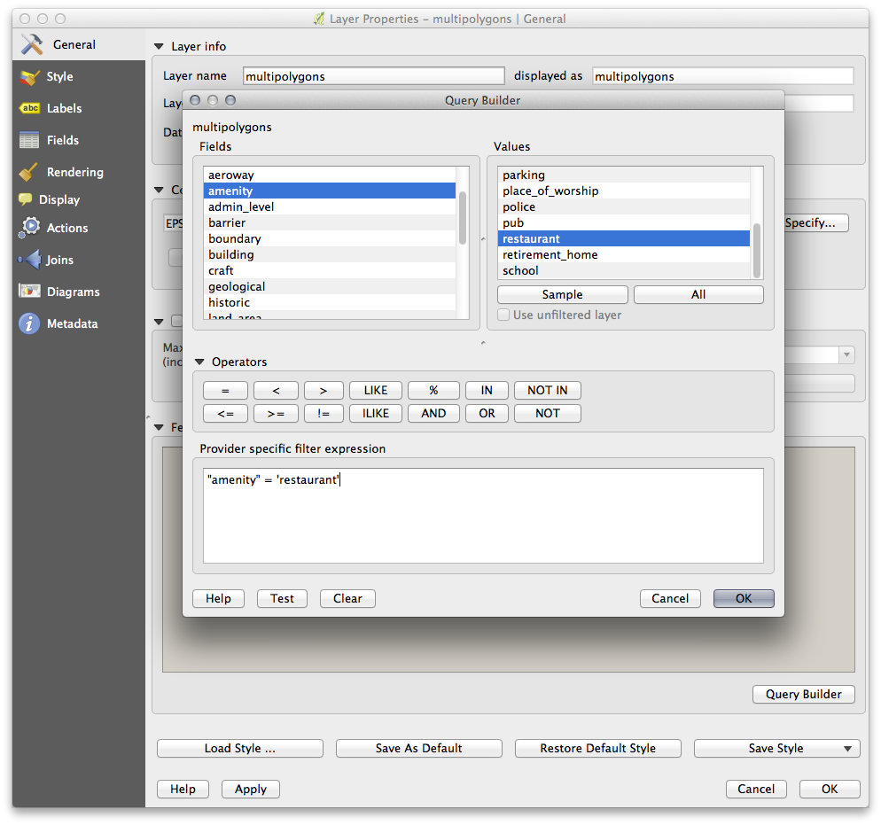
Using the Query Builder against the multipolygon layer,
create the following queries for the houses, schools,
restaurants and residential layers:
Once you have entered each query, click OK. You’ll see that the map
updates to show only the data you have selected. Since you need to use again
the multipolygon data from the OSM dataset, at this point, you can use one of
the following methods:
- Rename the filtered OSM layer and re-import the layer from
osm_data.osm, OR - Duplicate the filtered layer, rename the copy, clear the query and create your new query in the Query Builder.
Note
Although OSM’s building field has a house value, the
coverage in your area - as in ours - may not be complete. In our test
region, it is therefore more accurate to exclude all buildings which are
defined as anything other than house. You may decide to
simply include buildings which are defined as house and all other
values that have not a clear meaning like yes.
To create the roads layer, build this query against OSM’s lines
layer:
You should end up with a map which looks similar to the following:
18.9.2. Distance from High Schools
Your buffer dialog should look like this:
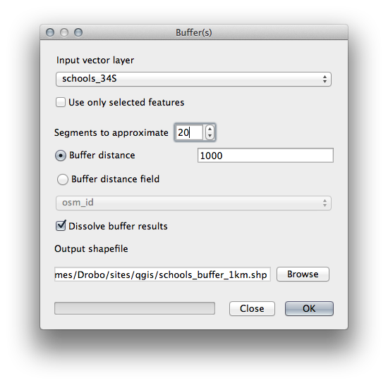
The Buffer distance is
1000meters (i.e.,1kilometer).The Segments to approximate value is set to
20. This is optional, but it’s recommended, because it makes the output buffers look smoother. Compare this: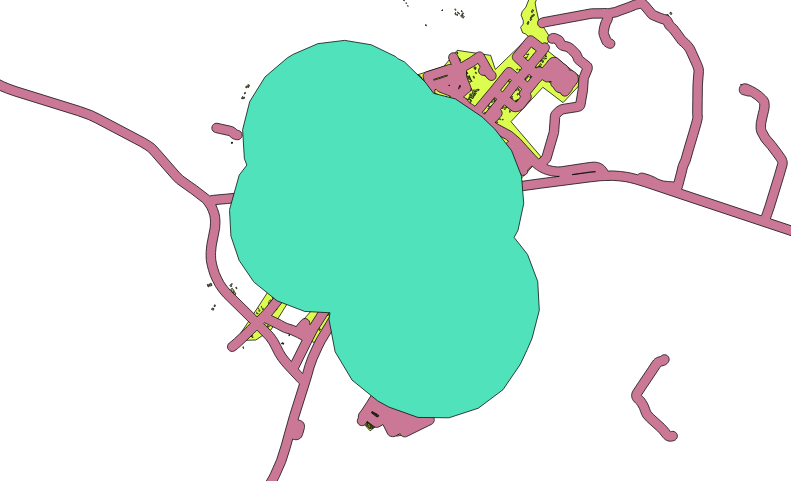
To this:
The first image shows the buffer with the Segments to approximate
value set to 5 and the second shows the value set to 20. In our
example, the difference is subtle, but you can see that the buffer’s edges are
smoother with the higher value.
Retour au texte
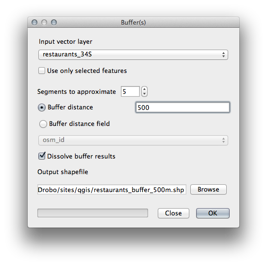
18.9.3. Distance from Restaurants
To create the new houses_restaurants_500m layer, we go through a two step
process:
First, create a buffer of 500m around the restaurants and add the layer to the map:
Next, select buildings within that buffer area:
Now save that selection to our new
houses_restaurants_500mlayer: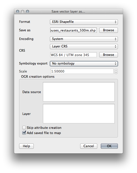
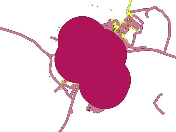
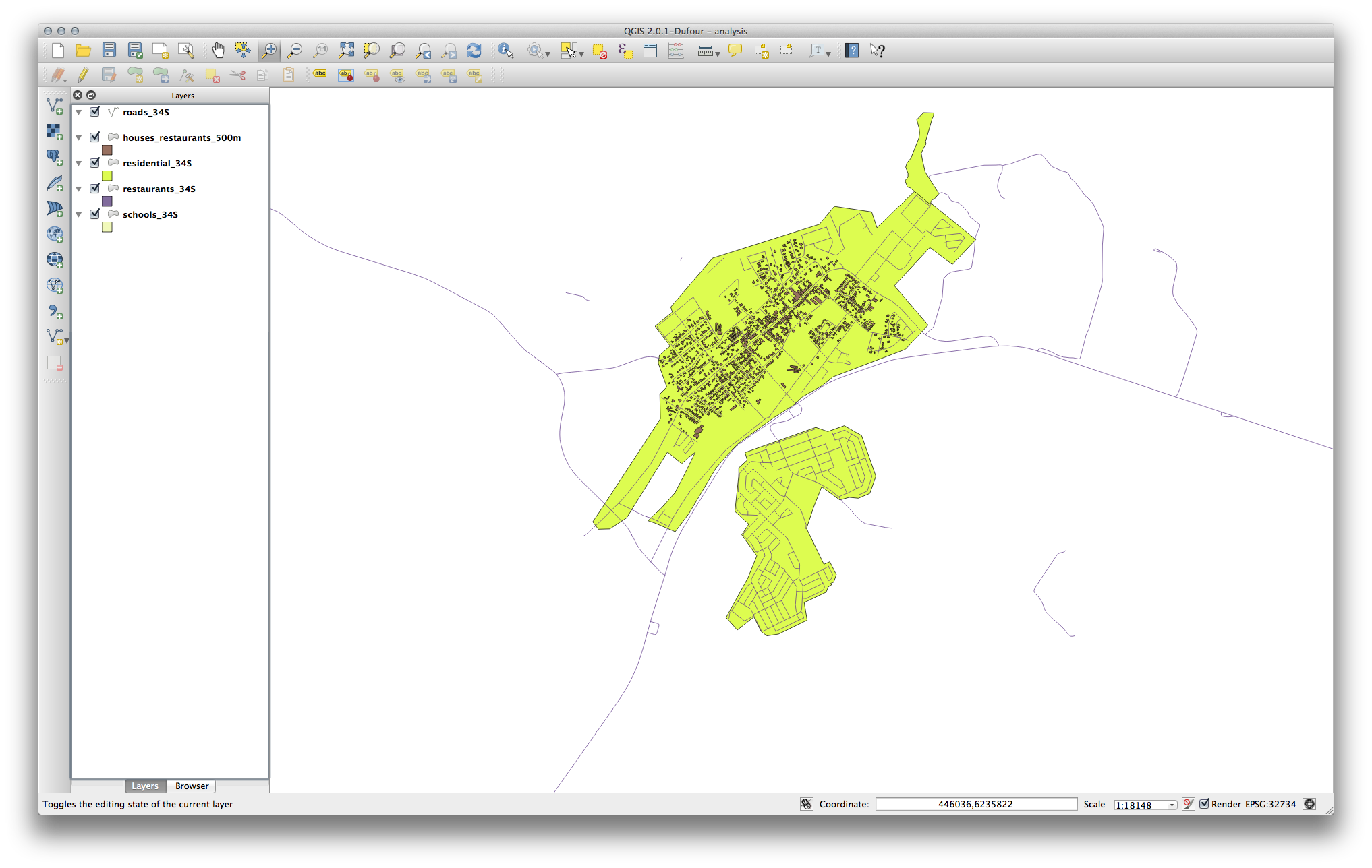
Your map should now show only those buildings which are within 50m of a road, 1km of a school and 500m of a restaurant:
18.10. Results For Raster Analysis
18.10.2. Calculate Slope (less than 2 and 5 degrees)
Set your Raster calculator dialog up like this:
For the 5 degree version, replace the
2in the expression and file name with5.
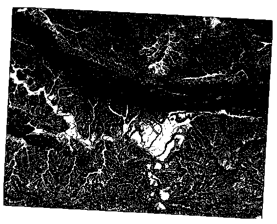
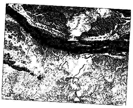
Vos résultats:
2 degrees:
5 degrees:
18.11. Results For Completing the Analysis
18.11.1. Raster to Vector
- Open the Query Builder by right-clicking on the all_terrain layer in the Layers list, select the General tab.
- Then build the query
"suitable" = 1. - Click OK to filter out all the polygons where this condition isn’t met.
When viewed over the original raster, the areas should overlap perfectly:

- You can save this layer by right-clicking on the all_terrain layer in the Layers list and choosing Save As..., then continue as per the instructions.
18.11.2. Inspecting the Results
You may notice that some of the buildings in your new_solution layer have
been “sliced” by the Intersect tool. This shows that only part of the
building - and therefore only part of the property - lies on suitable terrain.
We can therefore sensibly eliminate those buildings from our dataset
18.11.3. Refining the Analysis
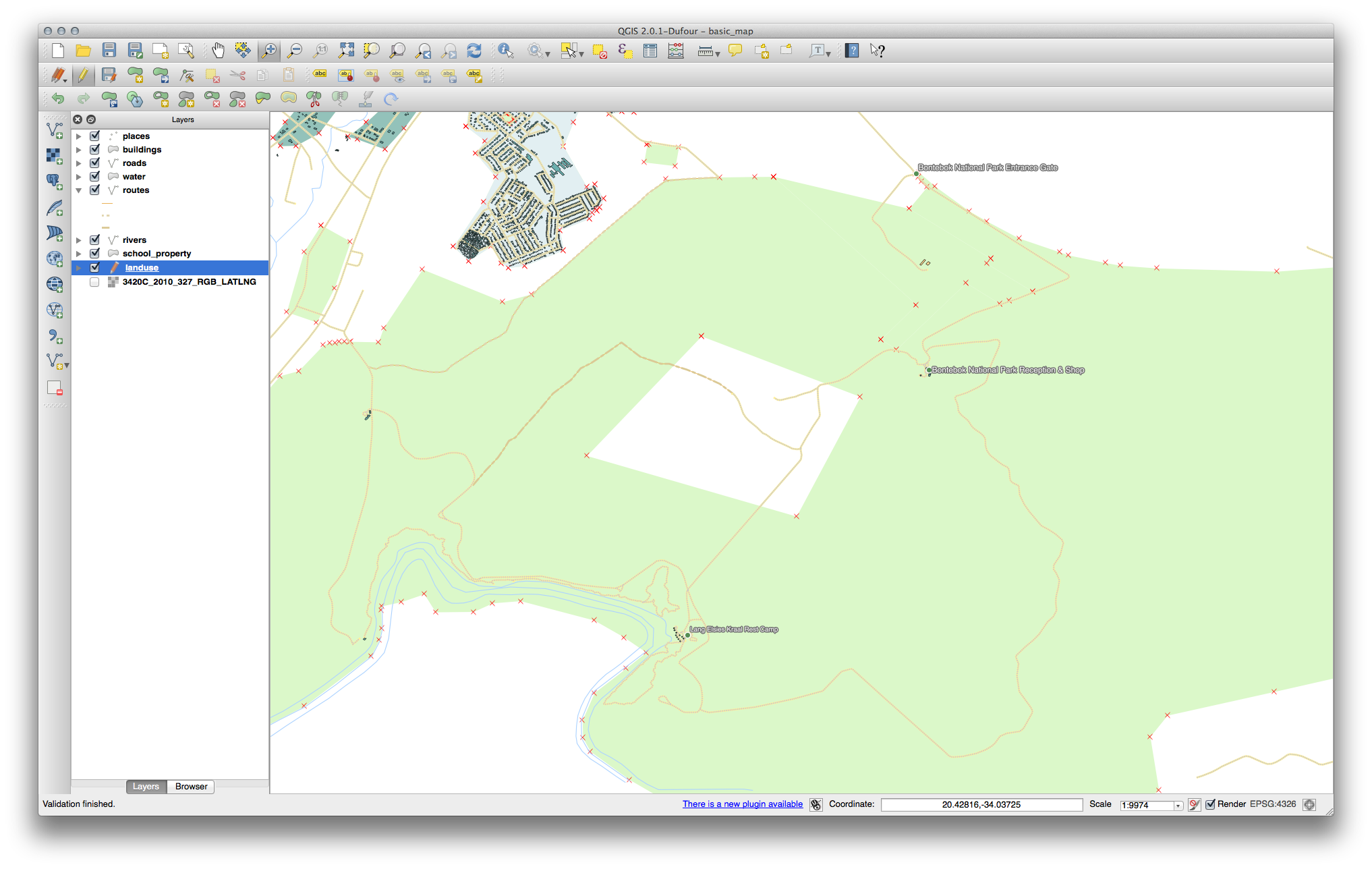
A ce stade, votre analyse devrait ressembler à peu près à ceci:
Consider a circular area, continuous for 100 meters in all directions.
If it is greater than 100 meters in radius, then subtracting 100 meters from its size (from all directions) will result in a part of it being left in the middle.
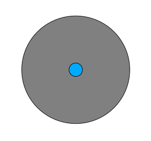
Therefore, you can run an interior buffer of 100 meters on your existing suitable_terrain vector layer. In the output of the buffer function, whatever remains of the original layer will represent areas where there is suitable terrain for 100 meters beyond.
To demonstrate:
Allez à Vecteur ‣ Outils de géotraitement ‣ Tampon(s) pour ouvrir la fenêtre Tampon(s).
Définissez-le comme ceci:
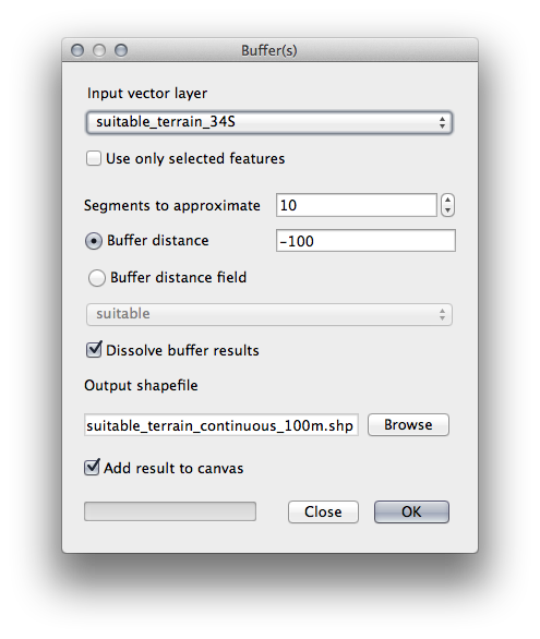
Use the suitable_terrain layer with
10segments and a buffer distance of-100. (The distance is automatically in meters because your map is using a projected CRS.)Save the output in
exercise_data/residential_development/assuitable_terrain_continuous100m.shp.If necessary, move the new layer above your original
suitable_terrainlayer.
Votre résultat ressemblera à peu près à ceci :
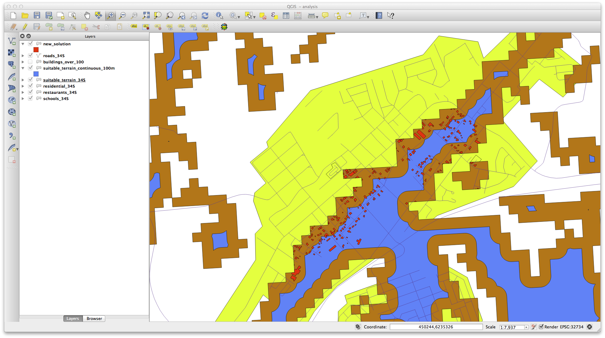
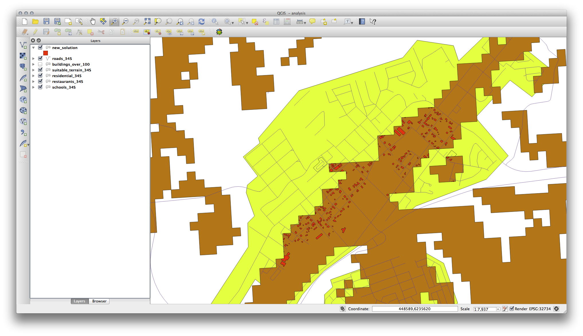
Maintenant, utilisez l’outil Sélection par localisation (Vecteur ‣ Outils de recherche ‣ Sélection par localisation).
Set up like this:
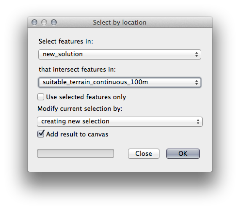
Select features in new_solution that intersect features in suitable_terrain_continuous100m.shp.
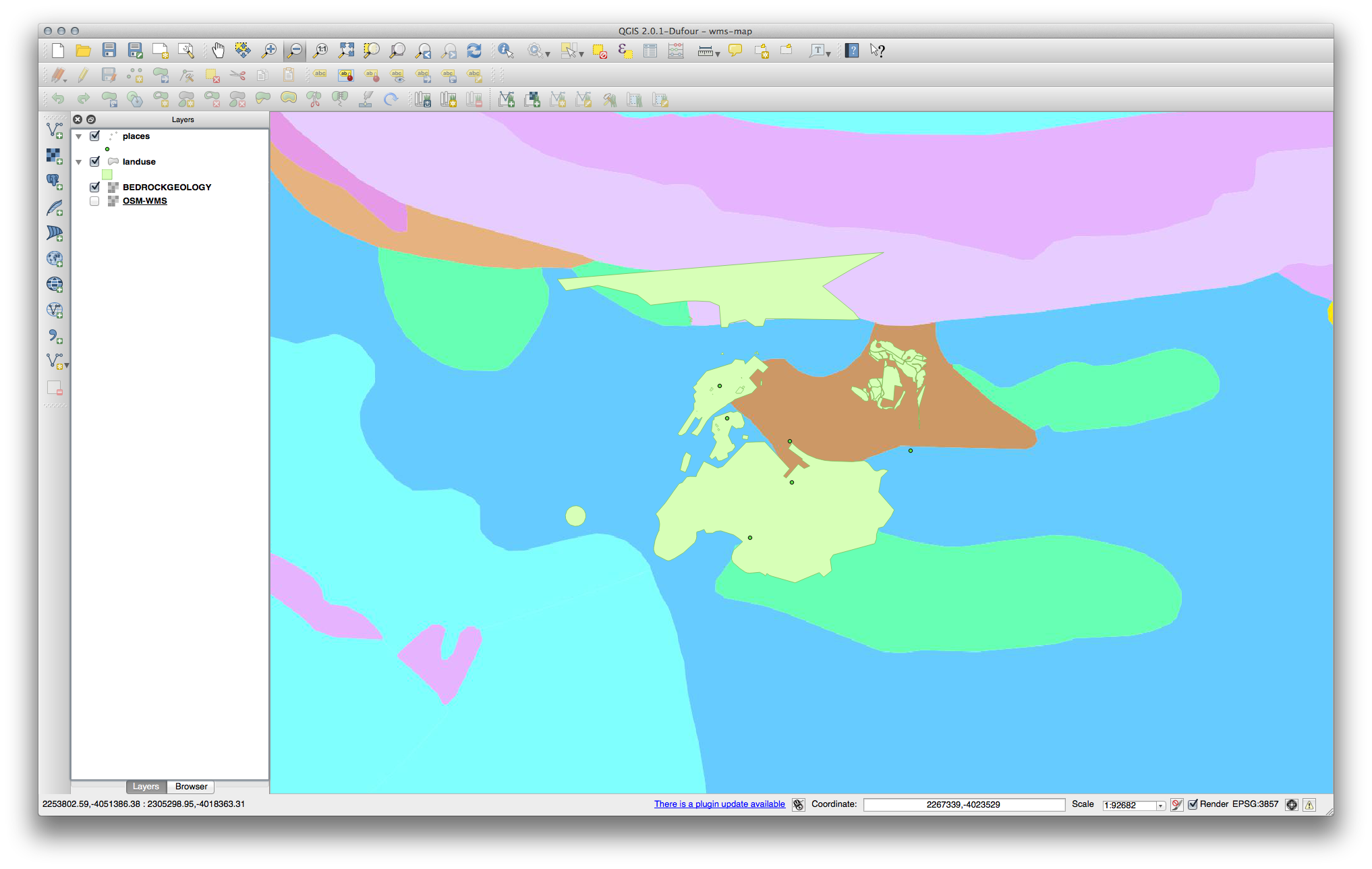
Voici le résultat:

The yellow buildings are selected. Although some of the buildings fall partly
outside the new suitable_terrain_continuous100m layer, they lie well
within the original suitable_terrain layer and therefore meet all of our
requirements.
- Save the selection under
exercise_data/residential_development/asfinal_answer.shp.
18.12. Results For WMS
18.12.1. Adding Another WMS Layer
Votre carte devrait ressembler à ceci (vous aurez peut-être besoin de réorganiser vos couches):
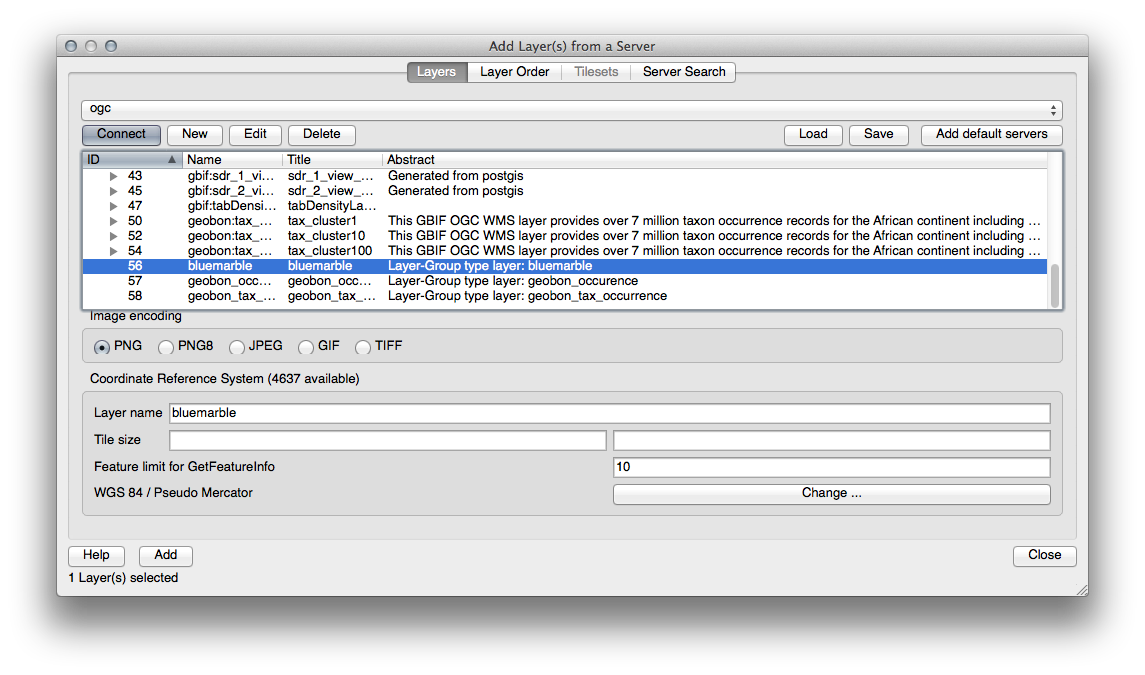
18.12.2. Ajout d’un Nouveau Serveur WMS
Use the same approach as before to add the new server and the appropriate layer as hosted on that server:

If you zoom into the Swellendam area, you’ll notice that this dataset has a low resolution:
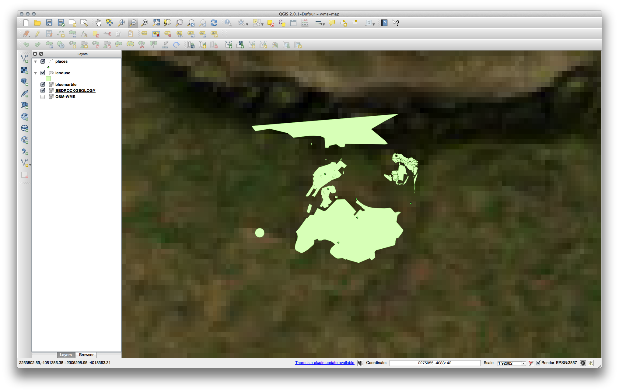
Therefore, it’s better not to use this data for the current map. The Blue Marble data is more suitable at global or national scales.
18.12.3. Finding a WMS Server
You may notice that many WMS servers are not always available. Sometimes this
is temporary, sometimes it is permanent. An example of a WMS server that worked
at the time of writing is the World Mineral Deposits WMS at
http://apps1.gdr.nrcan.gc.ca/cgi-bin/worldmin_en-ca_ows. It does not
require fees or have access constraints, and it is global. Therefore, it does
satisfy the requirements. Keep in mind, however, that this is merely an
example. There are many other WMS servers to choose from.
18.13. Results For Concepts de bases de données
18.13.1. Address Table Properties
For our theoretical address table, we might want to store the following properties:
House Number
Street Name
Suburb Name
City Name
Postcode
Country
When creating the table to represent an address object, we would create columns to represent each of these properties and we would name them with SQL-compliant and possibly shortened names:
house_number
street_name
suburb
city
postcode
country
18.13.2. Normalising the People Table
The major problem with the people table is that there is a single address field which contains a person’s entire address. Thinking about our theoretical address table earlier in this lesson, we know that an address is made up of many different properties. By storing all these properties in one field, we make it much harder to update and query our data. We therefore need to split the address field into the various properties. This would give us a table which has the following structure:
id |     name      | house_no |  street_name   |    city    |   phone_no
 --+---------------+----------+----------------+------------+-----------------
 1 | Tim Sutton    |     3    | Buirski Plein  | Swellendam | 071 123 123
 2 | Horst Duester |     4    | Avenue du Roix | Geneva     | 072 121 122
Note
In the next section, you will learn about Foreign Key relationships which could be used in this example to further improve our database’s structure.
18.13.3. Further Normalisation of the People Table
Our people table currently looks like this:
id |     name     | house_no | street_id |  phone_no
---+--------------+----------+-----------+-------------
 1 | Horst Duster |        4 |         1 | 072 121 122
The street_id column represents a ‘one to many’ relationship between the
people object and the related street object, which is in the streets
table.
One way to further normalise the table is to split the name field into first_name and last_name:
id | first_name | last_name  | house_no | street_id |  phone_no
---+------------+------------+----------+-----------+------------
 1 |    Horst   |   Duster   |     4    |     1     | 072 121 122
We can also create separate tables for the town or city name and country, linking them to our people table via ‘one to many’ relationships:
id | first_name | last_name | house_no | street_id | town_id | country_id
---+------------+-----------+----------+-----------+---------+------------
 1 |    Horst   |   Duster  |     4    |     1     |    2    |     1
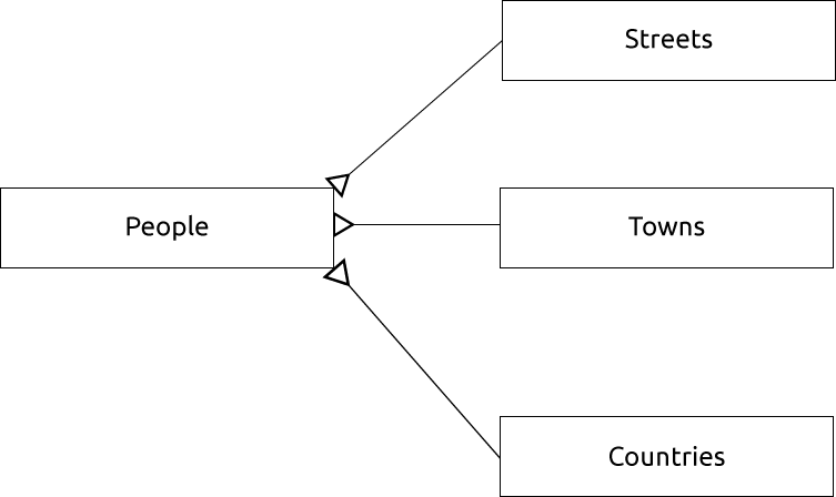
An ER Diagram to represent this would look like this:
18.13.4. Create a People Table
The SQL required to create the correct people table is:
create table people (id serial not null primary key,
                     name varchar(50),
                     house_no int not null,
                     street_id int not null,
                     phone_no varchar null );
The schema for the table (enter d people) looks like this:
Table "public.people"

Column     |         Type          |                      Modifiers
-----------+-----------------------+-------------------------------------
id         | integer               | not null default
           |                       | nextval('people_id_seq'::regclass)
name       | character varying(50) |
house_no   | integer               | not null
street_id  | integer               | not null
phone_no   | character varying     |
Indexes:
  "people_pkey" PRIMARY KEY, btree (id)
Note
For illustration purposes, we have purposely omitted the fkey constraint.
18.13.5. La commande DROP
The reason the DROP command would not work in this case is because the people table has a Foreign Key constraint to the streets table. This means that dropping (or deleting) the streets table would leave the people table with references to non-existent streets data.
Note
It is possible to ‘force’ the streets table to be deleted by using the CASCADE command, but this would also delete the people and any other table which had a relationship to the streets table. Use with caution!
18.13.6. Insert a New Street
The SQL command you should use looks like this (you can replace the street name with a name of your choice):
insert into streets (name) values ('Low Road');
18.13.7. Add a New Person With Foreign Key Relationship
Here is the correct SQL statement:
insert into streets (name) values('Main Road');
insert into people (name,house_no, street_id, phone_no)
  values ('Joe Smith',55,2,'072 882 33 21');
If you look at the streets table again (using a select statement as before),
you’ll see that the id for the Main Road entry is 2.
That’s why we could merely enter the number 2 above. Even though we’re
not seeing Main Road written out fully in the entry above, the
database will be able to associate that with the street_id value of
2.
Note
If you have already added a new street object, you might find
que la nouvelle Route Principale a un ID de 3 et non 2.
18.13.8. Return Street Names
Voici la syntaxe SQL correcte à utiliser:
select count(people.name), streets.name
from people, streets
where people.street_id=streets.id
group by streets.name;
Résultat:
count |    name
------+-------------
    1 | Low Street
    2 | High street
    1 | Main Road
(3 rows)
Note
Vous noterez que nous avons fait précéder les noms de champs par les noms de tables
- (par ex, people.name et streets.name). Ceci doit être fait chaque fois que
le nom d’un champ est ambigu (c’est-à-dire non unique dans l’ensemble des tables de la base de données).
18.14. Results For Requêtes Spatiales
18.14.1. Les Unités utilisées dans les requêtes spatiales
The units being used by the example query are degrees, because the CRS that the layer is using is WGS 84. This is a Geographic CRS, which means that its units are in degrees. A Projected CRS, like the UTM projections, is in meters.
Remember that when you write a query, you need to know which units the layer’s CRS is in. This will allow you to write a query that will return the results that you expect.
18.14.2. Création d’un Index Spatial
CREATE INDEX cities_geo_idx
  ON cities
  USING gist (the_geom);
18.15. Results For Geometry Construction
18.15.1. Creating Linestrings
alter table streets add column the_geom geometry;
alter table streets add constraint streets_geom_point_chk check
     (st_geometrytype(the_geom) = 'ST_LineString'::text OR the_geom IS NULL);
insert into geometry_columns values ('','public','streets','the_geom',2,4326,
     'LINESTRING');
create index streets_geo_idx
  on streets
  using gist
  (the_geom);
18.15.2. Linking Tables
delete from people;
alter table people add column city_id int not null references cities(id);
(capture cities in QGIS)
insert into people (name,house_no, street_id, phone_no, city_id, the_geom)
   values ('Faulty Towers',
           34,
           3,
           '072 812 31 28',
           1,
           'SRID=4326;POINT(33 33)');

insert into people (name,house_no, street_id, phone_no, city_id, the_geom)
   values ('IP Knightly',
           32,
           1,
           '071 812 31 28',
           1,
           'SRID=4326;POINT(32 -34)');

insert into people (name,house_no, street_id, phone_no, city_id, the_geom)
   values ('Rusty Bedsprings',
           39,
           1,
           '071 822 31 28',
           1,
           'SRID=4326;POINT(34 -34)');
Si vous obtenez le message d’erreur suivant:
ERROR:  insert or update on table "people" violates foreign key constraint
        "people_city_id_fkey"
DETAIL: Key (city_id)=(1) is not present in table "cities".
then it means that while experimenting with creating polygons for the
cities table, you must have deleted some of them and started over. Just
check the entries in your cities table and use any id which exists.
18.16. Results For Simple Feature Model
18.16.1. Populating Tables
create table cities (id serial not null primary key,
                     name varchar(50),
                     the_geom geometry not null);
 alter table cities
 add constraint cities_geom_point_chk
 check (st_geometrytype(the_geom) = 'ST_Polygon'::text );
18.16.2. Populate the Geometry_Columns Table
insert into geometry_columns values
      ('','public','cities','the_geom',2,4326,'POLYGON');
18.16.3. Adding Geometry
select people.name,
       streets.name as street_name,
       st_astext(people.the_geom) as geometry
from   streets, people
where  people.street_id=streets.id;
Résultat:
     name     | street_name |   geometry
--------------+-------------+---------------
 Roger Jones  | High street |
 Sally Norman | High street |
 Jane Smith   | Main Road   |
 Joe Bloggs   | Low Street  |
 Fault Towers | Main Road   | POINT(33 -33)
(5 rows)
Comme vous pouvez le voir, notre contrainte autorise l’ajout de valeurs nulles dans la base de données.