2. Lesson: Analyse Vectorielle¶

2.1. The GIS Process¶

Avant de commencer, il serait utile de donner un bref aperçu d’un processus qui peut être utilisé pour résoudre les problèmes en SIG. Les étapes à suivre à ce sujet sont :

1. Énoncer le problème

2. Obtenir les données

3. Analyser le problème

4. Présenter les résultats

2.2. Le problème¶

Nous allons commencer le processus en décidant d’un problème à résoudre. Par exemple, vous êtes un agent immobilier et vous recherchez une propriété résidentielle à Swellendam pour des clients dont les critères sont les suivants:

1. Elle doit être en Swellendam.

2. Elle doit être à une distance raisonnable en voiture (disons 1km) d’une école

3. Elle doit avoir une taille de plus de 100m²

4. A moins de 50m d’une route principale

5. A moins de 500m d’un restaurant.

2.3. Les données¶

Pour répondre à ces questions, nous aurons besoin des données suivantes:

1. Les propriétés résidentielles (constructions) dans le périmètre,

2. Les routes dans et autour de la ville,

3. La localisation des écoles et des restaurants,

4. La taille des constructions.

Toutes ces données sont disponibles via OSM et vous pourriez trouver que le jeu de données que vous utilisez depuis le début de ce manuel peut aussi l’être pour cette leçon. Toutefois, afin de nous assurer que nous avons toutes les données requises, nous allons re-télécharger les données depuis OSM à l’aide de l’outil de téléchargement de données OSM intégré à QGIS.

2.4. Follow Along: Démarrer un Projet¶

• Démarrez un nouveau projet QGIS.

• Utilisez l’outil de téléchargement de données OpenStreetMap accessible via le menu Vector -> OpenStreeMap pour télécharger les données de la région que vous avez choisie.

• Sauvegardez les données sous osm_data.osm dans votre dossier exercise_data.

• Notez que le format osm est de type vectoriel. Ajoutez donc cette donnée en tant que couche vectorielle via le menu Couche -> Ajouter une couche vecteur..., parcourez l’arborescence jusqu’à votre nouveau fichier osm_data.osm. Il vous faudra surement:

sélectionner Tous les fichiers comme format de fichier.

• Sélectionnez osm_data.osm et cliquez sur Ouvrir

• Dans la fenêtre qui s’ouvre, sélectionnez toutes les couches, à l’exception de other_relations et multilinestrings:

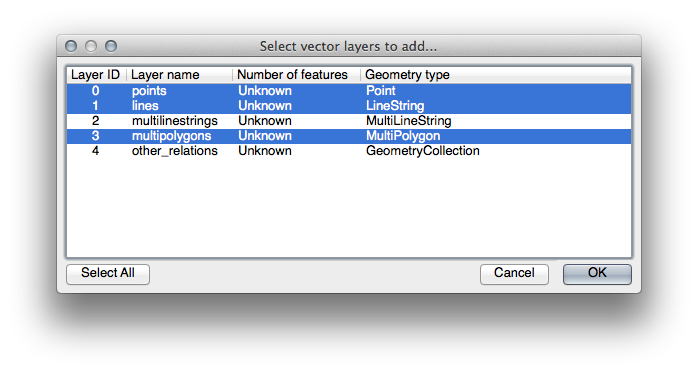
Les données OSM seront importées en couches séparées dans votre carte.

The data you just downloaded from OSM is in a geographic coordinate system, WGS84, which uses latitude and longitude coordinates, as you know from the previous lesson. You also learnt that to calculate distances in meters, we need to work with a projected coordinate system. Start by setting your project’s coordinate system to a suitable CRS for your data, in the case of Swellendam, WGS 84 / UTM zone 34S:

• Open the Project Properties dialog, select CRS and filter the list to find WGS 84 / UTM zone 34S.

• Cliquez sur OK.

We now need to extract the information we need from the OSM dataset. We need to end up with layers representing all the houses, schools, restaurants and roads in the region. That information is inside the multipolygons layer and can be extracted using the information in its Attribute Table. We’ll start with the schools layer:

• Right-click on the multipolygons layer in the Layers list and open the Layer Properties.

• Rendez-vous sur l’onglet Général.

• Under Feature subset click on the [Query Builder] button to open the Query builder dialog.
• In the Fields list on the left of this dialog until you see the field amenity.

• Cliquez dessus une fois.

• Cliquez sur le bouton Tout en-dessous de la liste Valeurs:

Maintenant, nous devons dire à QGIS de ne nous montrer que les polygones dont la valeur amenity est égale à school.

• Double-cliquez sur le mot amenity dans la liste Champs.

• Watch what happens in the Provider specific filter expression

field below:

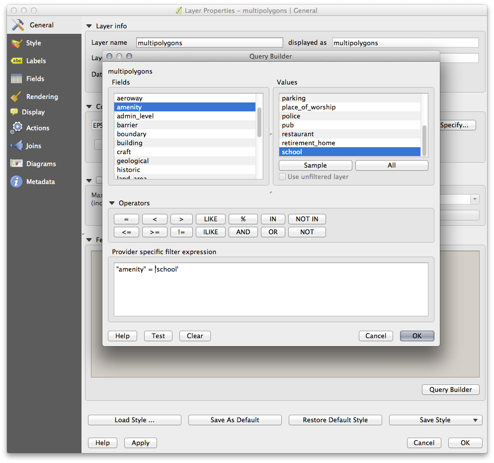
The word "amenity" has appeared. To build the rest of the query:

• Click the = button (under Operators).
• Double-click the value school in the Values list.

• Cliquez sur OK deux fois.

This will filter OSM’s multipolygon layer to only show the schools in your region. You can now either:

• Rename the filtered OSM layer to schools and re-import the multipolygons layer from osm_data.osm, OR
• Duplicate the filtered layer, rename the copy, clear the Query Builder and create your new query in the Query Builder.

2.5. Try Yourself Extract Required Layers from OSM¶

Using the above technique, use the Query Builder tool to extract the remaining data from OSM to create the following layers:

• roads (from OSM’s lines layer)
• restaurants (from OSM’s multipolygons layer)
• houses (from OSM’s multipolygons layer)

You may wish to re-use the roads.shp layer you created in earlier lessons.

Vérifiez vos résultats

• Enregistrez votre carte sous analysis.qgs dans le dossier exercise_data.

• In your operating system’s file manager, create a new folder under exercise_data and call it residential_development. This is where you’ll save the datasets that will be the results of the analysis functions.

2.6. Try Yourself Find important roads¶

Some of the roads in OSM’s dataset are listed as unclassified, tracks, path and footway. We want to exclude these from our roads dataset.

• Open the Query Builder for the roads layer, click Clear and build the following query:

  "highway"  != 'NULL' AND "highway" != 'unclassified' AND "highway" != 'track' AND "highway" != 'path' AND "highway" != 'footway'

You can either use the approach above, where you double-clicked values and clicked buttons, or you can copy and paste the command above.

This should immediately reduce the number of roads on your map:

2.7. Try Yourself Convert Layers’ CRS¶

Because we are going to be measuring distances within our layers, we need to change the layers’ CRS. To do this, we need to select each layer in turn, save the layer to a new shapefile with our new projection, then import that new layer into our map.

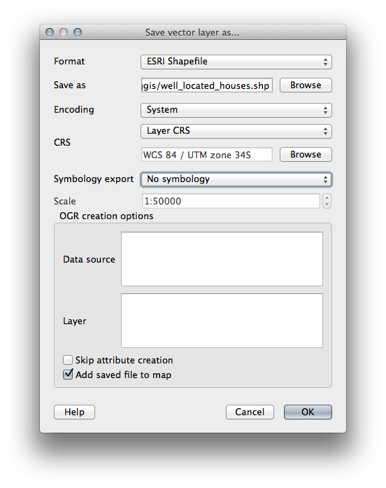
• Right click the roads layer in the Layers panel.

• Cliquez sur Sauvegarder sous...

• In the Save Vector As dialog, choose the following settings and click Ok (making sure you select Add saved file to map):

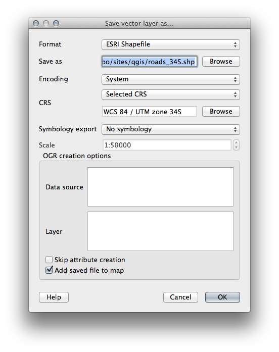
Une nouvelle couche shapefile sera créée et ajoutée à la carte.

• Supprimez l’ancienne couche roads.

Repeat this process for each layer, creating a new shapefile and layer with “_34S” appended to the original name and removing each of the old layers.

Once you have completed the process for each layer, right click on any layer and click Zoom to layer extent to focus the map to the area of interest.

Now that we have converted OSM’s data to a UTM projection, we can begin our calculations.

2.8. Follow Along: Analyzing the Problem: Distances From Schools and Roads¶

QGIS allows you to calculate distances from any vector object.

• Make sure that only the roads_34S and houses_34S layers are visible, to simplify the map while you’re working.

• Cliquez sur l’outil Vecteur ‣ Outils de géotraitement ‣ Tampon(s):

Une nouvelle fenêtre s’ouvre.

• Set it up like this:

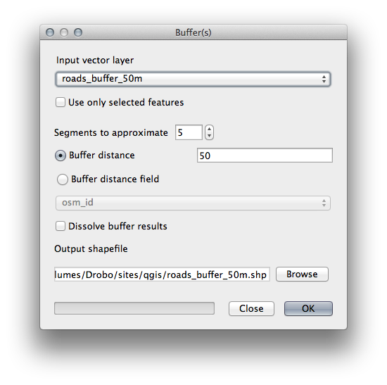
The Buffer distance is in meters because our input dataset is in a Projected Coordinate System that uses meter as its basic measurement unit. This is why we needed to use projected data.

• Save the resulting layer under exercise_data/residential_development/ as roads_buffer_50m.shp.

• Cliquez sur OK et il créera une zone tampon.

• When it asks you if it should “add the new layer to the TOC”, click Yes. (“TOC” stands for “Table of Contents”, by which it means the Layers list).

• Fermez la fenêtre Tampon(s).

Maintenant, votre carte devrait ressembler à peu près à ceci:

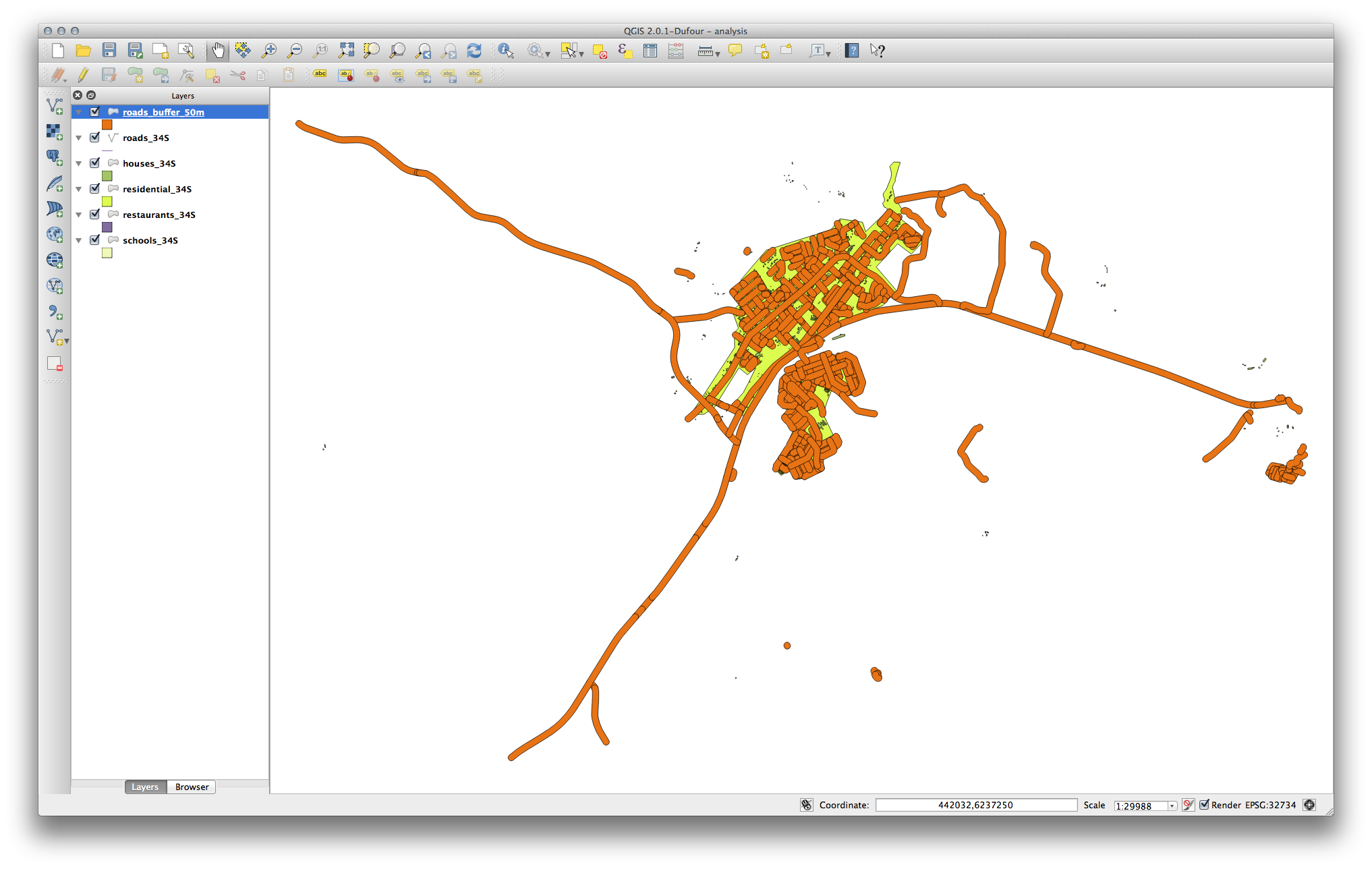
If your new layer is at the top of the Layers list, it will probably obscure much of your map, but this gives us all the areas in your region which are within 50m of a road.

However, you’ll notice that there are distinct areas within our buffer, which correspond to all the individual roads. To get rid of this problem, remove the layer and re-create the buffer using the settings shown here:

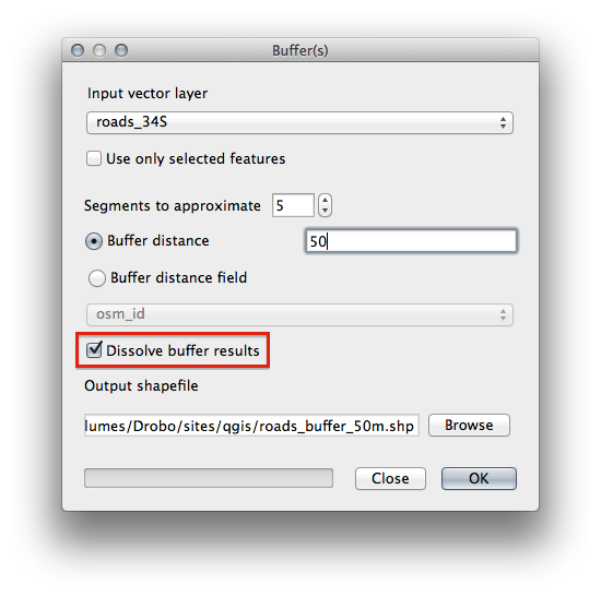
• Note that we’re now checking the Dissolve buffer results box.
• Save the output under the same name as before (click Yes when it asks your permission to overwrite the old one).
• Click OK and close the Buffer(s) dialog again.

Once you’ve added the layer to the Layers list, it will look like this:

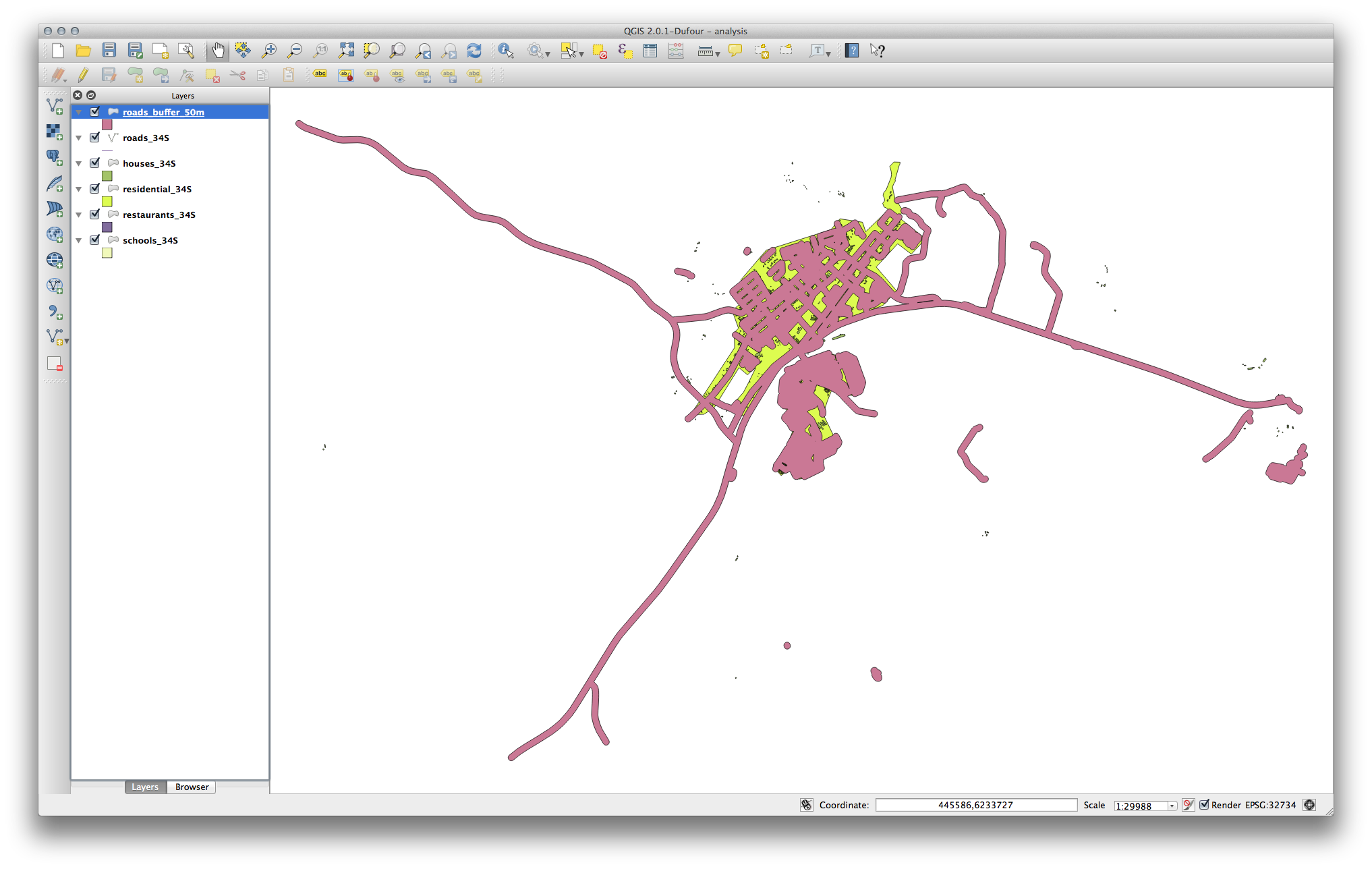
Now there are no unnecessary subdivisions.

2.9. Try Yourself Distance from schools¶

• Use the same approach as above and create a buffer for your schools.

It needs to be 1 km in radius, and saved under the usual directory as schools_buffer_1km.shp.

Vérifiez vos résultats

2.10. Follow Along: Overlapping Areas¶

Now we have areas where the road is 50 meters away and there’s a school within 1 km (direct line, not by road). But obviously, we only want the areas where both of these criteria are satisfied. To do that, we’ll need to use the Intersect tool. Find it under Vector ‣ Geoprocessing Tools ‣ Intersect. Set it up like this:

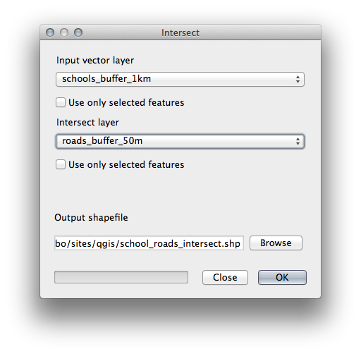
The two input layers are the two buffers; the save location is as usual; and the file name is road_school_buffers_intersect.shp. Once it’s set up like this, click OK and add the layer to the Layers list when prompted.

In the image below, the blue areas show us where both distance criteria are satisfied at once!

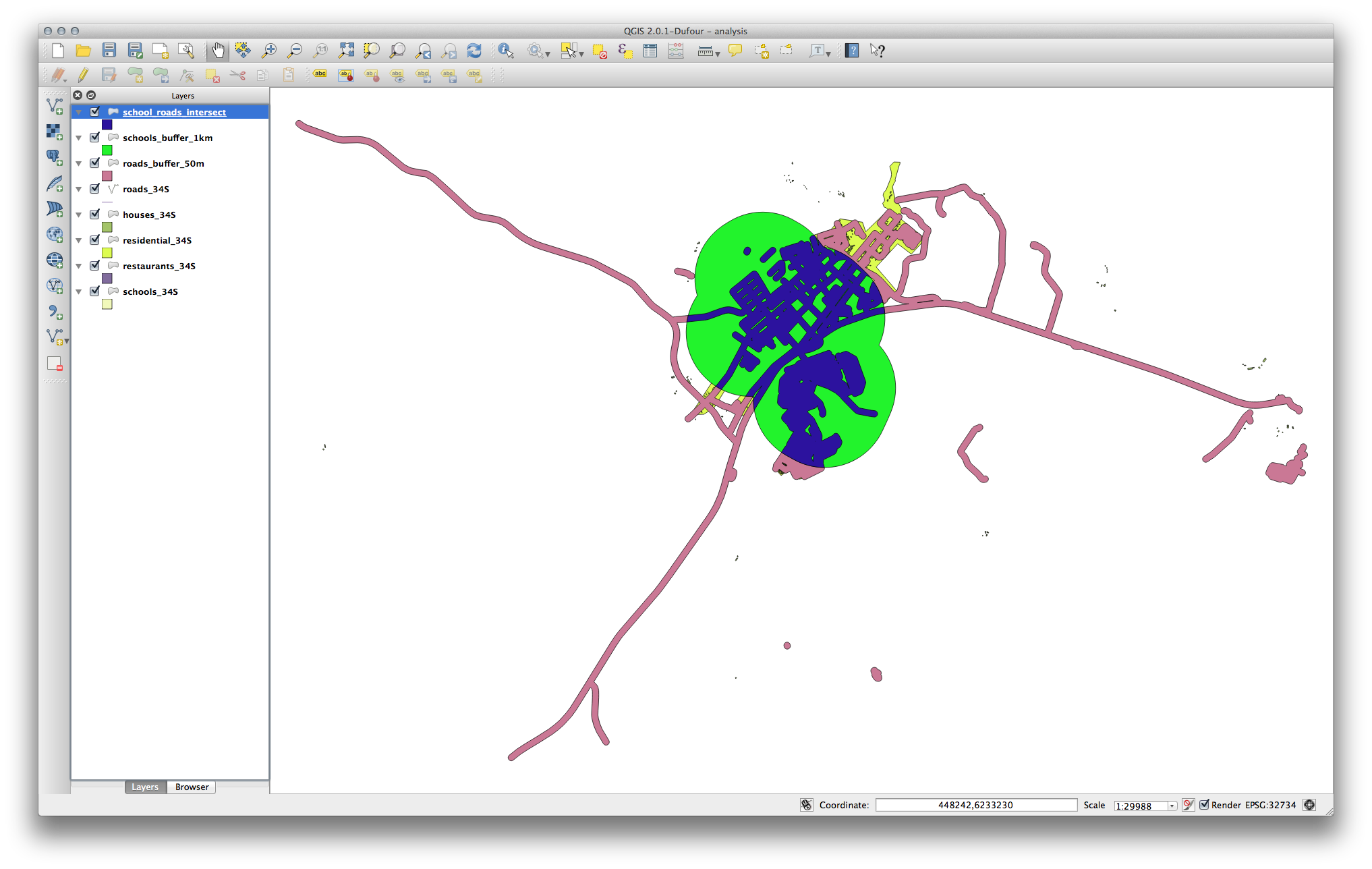
You may remove the two buffer layers and only keep the one that shows where they overlap, since that’s what we really wanted to know in the first place:

2.11. Follow Along: Select the Buildings¶

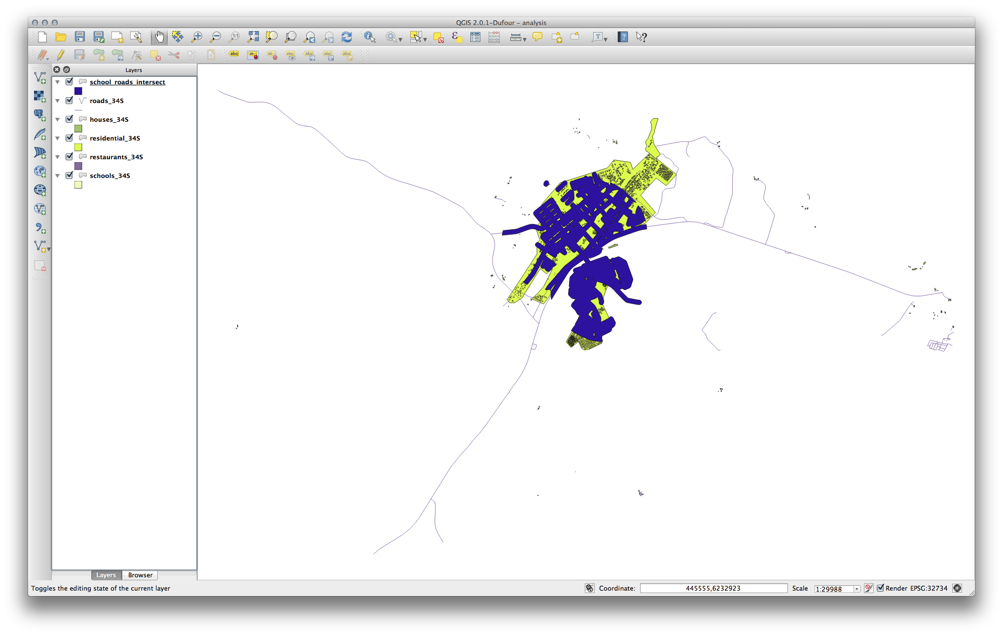
Now you’ve got the area that the buildings must overlap. Next, you want to select the buildings in that area.

• Cliquez sur l’entrée du menu Vecteur ‣ Outils de recherche ‣ Sélection par localisation. Une fenêtre apparaîtra.

• Set it up like this:

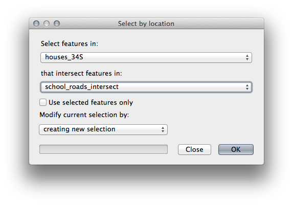
• Cliquez sur OK puis sur Fermer.

• You’ll probably find that not much seems to have changed. If so, move the school_roads_intersect layer to the bottom of the layers list, then zoom in:

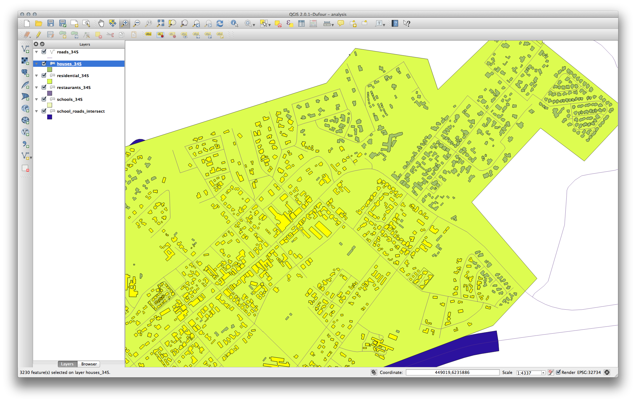
The buildings highlighted in yellow are those which match our criteria and are selected, while the buildings in green are those which do not. We can now save the selected buildings as a new layer.

• Right-click on the houses_34S layer in the Layers list.

• Sélectionnez Sauvegarder la sélection sous....

• Set the dialog up like this:

• The file name is well_located_houses.shp.

• Cliquez sur OK.

Now you have the selection as a separate layer and can remove the houses_34S layer.

2.12. Try Yourself Further Filter our Buildings¶

We now have a layer which shows us all the buildings within 1km of a school and within 50m of a road. We now need to reduce that selection to only show buildings which are within 500m of a restaurant.

Using the processes described above, create a new layer called houses_restaurants_500m which further filters your well_located_houses layer to show only those which are within 500m of a restaurant.

Vérifiez vos résultats

2.13. Follow Along: Select Buildings of the Right Size¶

To see which buildings are the correct size (more than 100 square metres), we first need to calculate their size.

• Open the attribute table for the houses_restaurants_500m layer.
• Enter edit mode and open the field calculator.
• Set it up like this:

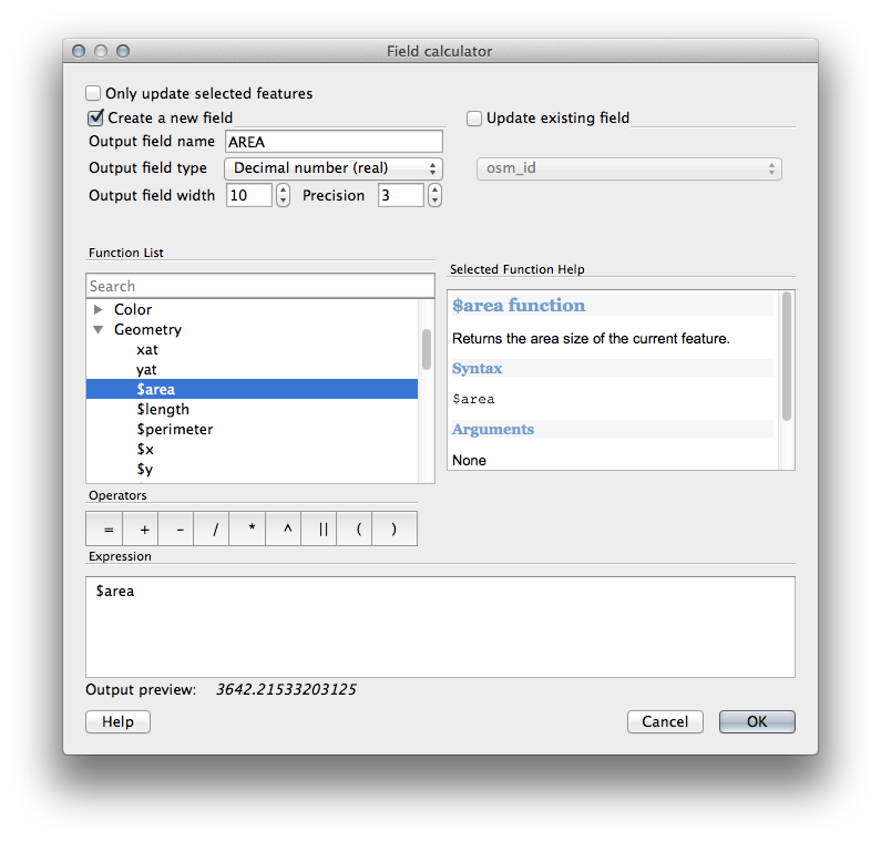
• Si vous ne trouvez pas AREA dans la liste, essayez donc de créer un nouveau champ comme vous l’avez fait dans la précédente leçon de ce module.

• Cliquez sur OK.

• Scroll to the right of the attribute table; your AREA field now has areas in metres for all the buildings in your houses_restaurants_500m layer.
• Click the edit mode button again to finish editing, and save your edits when prompted.
• Build a query as earlier in this lesson:

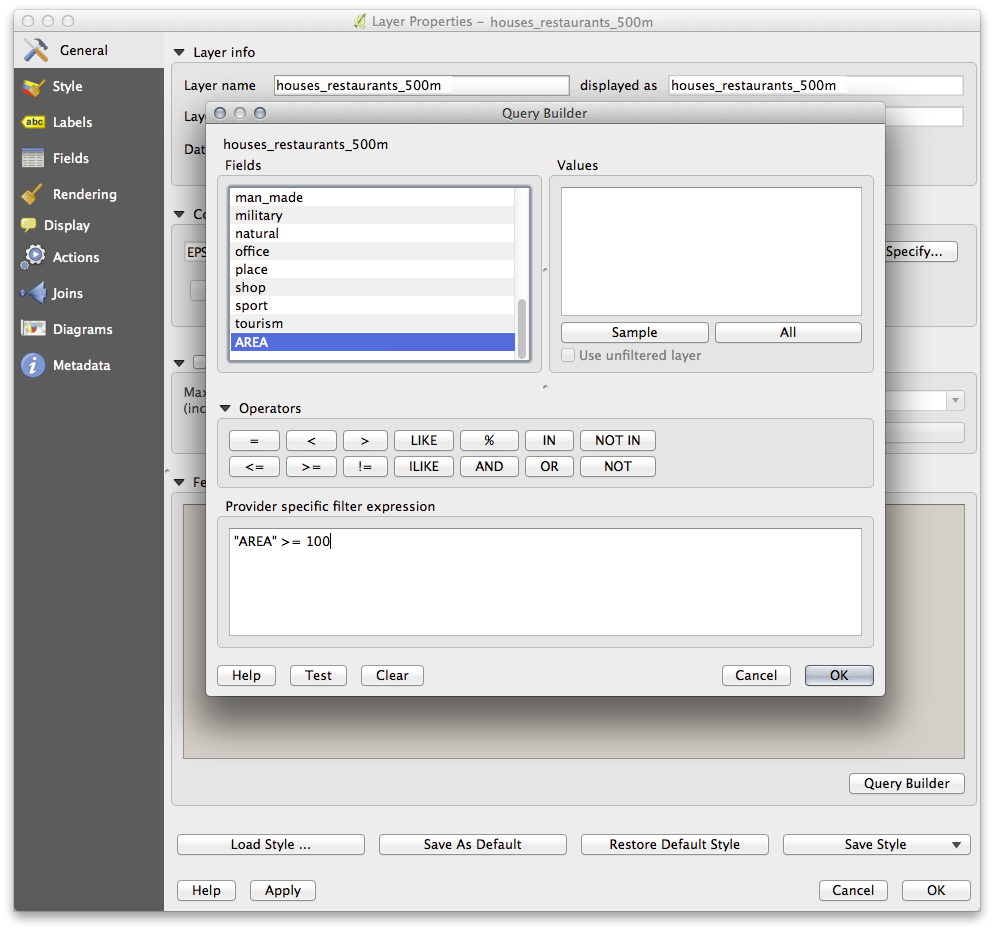
• Click OK. Your map should now only show you those buildings which match our starting criteria and which are more than 100m squared in size.

2.14. Try Yourself¶

• Save your solution as a new layer, using the approach you learned above for doing so. The file should be saved under the usual directory, with the name solution.shp.

2.15. In Conclusion¶

Using the GIS problem-solving approach together with QGIS vector analysis tools, you were able to solve a problem with multiple criteria quickly and easily.

2.16. What’s Next?¶

In the next lesson, we’ll look at how to calculate the shortest distance along the road from one point to another.