7.2. Lesson: 벡터 분석

벡터 데이터를 분석해서 서로 다른 피처들이 공간 안에서 어떻게 상호작용하는지 밝힐 수 있습니다. GIS에는 서로 다른 많은 분석 관련 기능들이 있는데, 모든 기능을 다 살펴보지는 않을 것입니다. 그보다는 문제를 제시하고 QGIS가 제공하는 도구들을 써서 그 문제를 해결하는 방식을 사용할 것입니다.

이 강의의 목표: 문제를 제시하고, 분석 도구를 써서 해결하기

7.2.1. GIS 처리 과정

시작하기 전 GIS 문제를 해결하는 데 사용할 수 있는 처리 과정을 간략히 살펴보는 것이 좋을 것입니다. 다음과 같은 처리 과정을 거칩니다.

1. 문제를 정의

2. 데이터 획득

3. 문제를 분석

4. 결과를 표출

7.2.2. The Problem

해결해야 할 문제를 결정하는 것으로 처리 과정을 시작합시다. 예를 들어 여러분이 부동산 업자인데 다음 기준을 가진 고객을 위해 Swellendam 에 있는 거주지를 찾고 있다고 해봅시다.

1. It needs to be in Swellendam

2. It must be within reasonable driving distance of a school (say 1km)

3. It must be more than 100m squared in size

4. Closer than 50m to a main road

5. Closer than 500m to a restaurant

7.2.3. The Data

이 문제들을 해결하려면 다음 데이터들이 필요합니다.

1. The residential properties (buildings) in the area

2. The roads in and around the town

3. The location of schools and restaurants

4. The size of buildings

All of this data is available through OSM and you should find that the dataset you have been using throughout this manual can also be used for this lesson.

If you want to download data from another area jump to Introduction Chapter section to read how to do it.

참고

OSM 다운로드는 일관된 데이터 항목을 가지고 있지만, 커버리지 및 세부 내용은 다를 수 있습니다. 예를 들어 여러분이 선택한 지역에 식당 정보가 없다면, 다른 지역을 선택해야 할 수도 있습니다.

7.2.4. Follow Along: Start a Project and get the Data

We first need to load the data to work with.

1. Start a new QGIS project

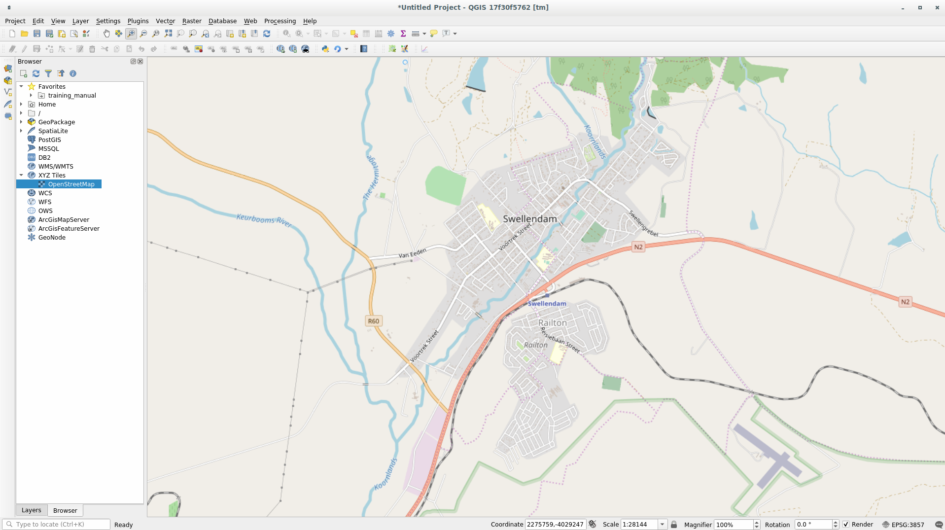
2. If you want you can add a background map. Open the Browser and load the OSM background map from the XYZ Tiles menu.

   

3. In the training_data.gpkg Geopackage database load all the files we will use in this chapter:

   1. landuse

   2. buildings

   3. roads

   4. restaurants

   5. schools

4. Zoom to the layer extent to see Swellendam, South Africa

Before proceeding we should filter the roads layer in order to have only some specific road types to work with.

Some of the roads in OSM dataset are listed as unclassified, tracks, path and footway. We want to exclude these from our dataset and focus on the other road types, more suitable for this exercise.

Moreover, OSM data might not be updated everywhere and we will also exclude NULL values.

1. Right click on the roads layer and choose Filter….

2. In the dialog that pops up we can filter these features with the following expression:

   "highway" NOT IN ('footway','path','unclassified','track') OR "highway" != NULL
   

   The concatenation of the two operators NOT and IN means to exclude all the unwanted features that have these attributes in the highway field.

   != NULL combined with the OR operator is excluding roads with no values in the highway field.

   You will note the icon next to the roads layer that helps you remember that this layer has a filter activated and not all the features are available in the project.

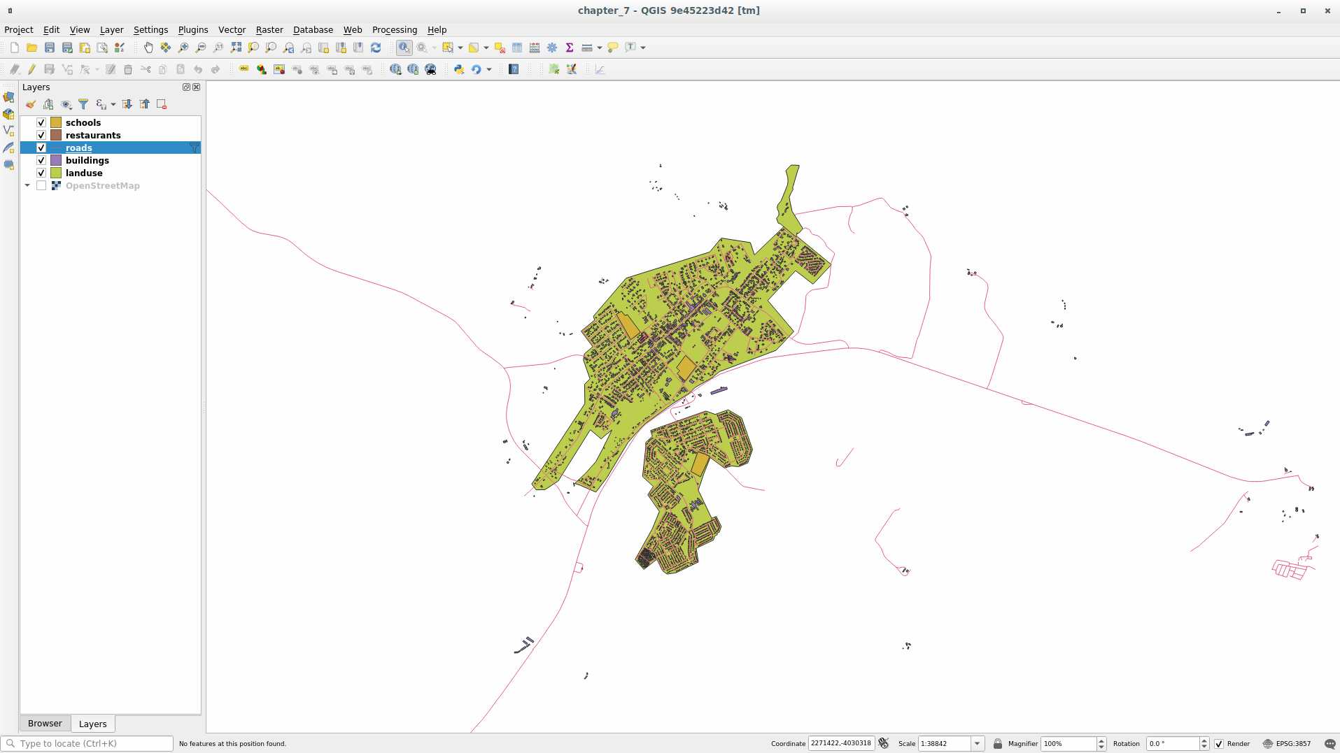
The map with all the data should look like the following one:

7.2.5. Try Yourself 레이어 CRS 변환

Because we are going to be measuring distances within our layers, we need to change the layers〉 CRS. To do this, we need to select each layer in turn, save the layer to a new one with our new projection, then import that new layer into our map.

You have many different options, e.g. you can export each layer as a new Shapefile, you can append the layers to an existing GeoPackage file or you can create another GeoPackage file and fill it with the new reprojected layers. We will show the last option so the training_data.gpkg will remain clean. But feel free to choose the best workflow for yourself.

참고

이 예제에서는 WGS 84 / UTM zone 34S CRS를 사용할 것이지만, 여러분이 다른 지역을 선택했다면 해당 지역에 더 적합한 UTM CRS를 사용할 수도 있습니다.

1. Right click the roads layer in the Layers panel;

2. Click Export –> Save Features As…;

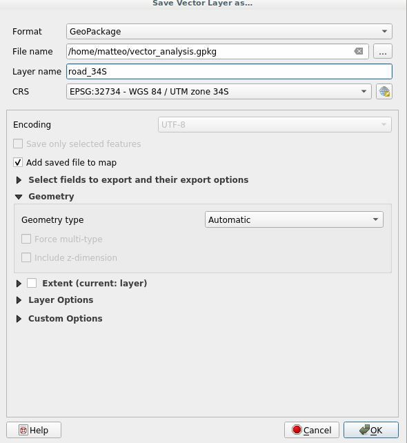
3. In the Save Vector Layer As dialog choose GeoPackage as Format;

4. Click on … of File name parameter and name the new GeoPackage as vector_analysis;

5. Change the Layer name as roads_34S;

6. Change the CRS parameter to WGS 84 / UTM zone 34S;

7. Finally click on OK:

   

   This will create the new GeoPackage database and fill it with the roads_34S layer.

8. Repeat this process for each layer, creating a new layer in the vector_analysis.gpkg GeoPackage file with _34S appended to the original name and removing each of the old layers from the project.

   참고

   When you choose to save a layer to an existing GeoPackage, QGIS will append that layer in the GeoPackage.

9. 각 레이어에 대해 이 과정을 완료한 다음 아무 레이어나 오른쪽 클릭하고 Zoom to layer extent 를 클릭해서 관심지역으로 맵을 이동시킵니다.

이제 OSM 데이터에 UTM 투영체를 적용시켰으니, 계산을 시작할 수 있습니다.

7.2.6. Follow Along: 문제 분석: 학교 및 도로부터의 거리

QGIS는 어떤 벡터 오브젝트부터의 거리도 계산할 수 있습니다.

1. Make sure that only the roads_34S and buildings_34S layers are visible, to simplify the map while you’re working

2. Click on the Processing ‣ Toolbox to open the analytical core of QGIS. Basically: all algorithms (for vector and raster) analysis are available within this toolbox.

3. We start by calculating the area around the roads_34S by using the Buffer algorithm. You can find it expanding the Vector Geometry group.

   

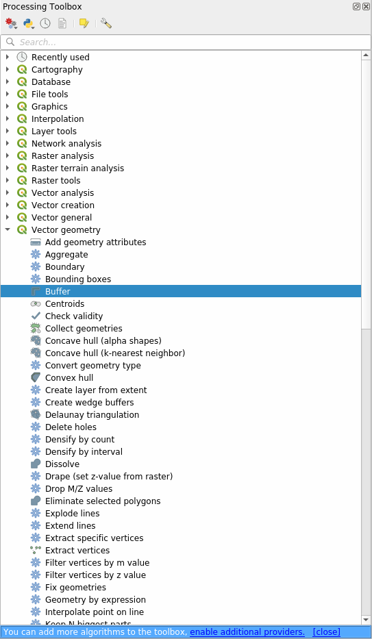
   Or you can type buffer in the search menu in the upper part of the toolbox: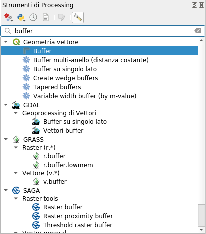

   

4. Double click on it to open the algorithm dialog

5. Set it up like this

   

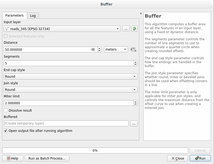
6. The default Distance is in meters because our input dataset is in a Projected Coordinate System that uses meter as its basic measurement unit. You can use the combo box to choose other projected units like kilometers, yards, etc.

   참고

   If you are trying to make a buffer on a layer with a Geographical Coordinate System, Processing will warn you and suggest to reproject the layer to a metric Coordinate System.

7. By default Processing creates temporary layers and adds them to the Layers panel. You can also append the result to the GeoPackage database by:

   1. clicking on the … button and choose Save to GeoPackage…

   2. naming the new layer roads_buffer_50m

   3. and saving it in the vector_analysis.gpkg file

   

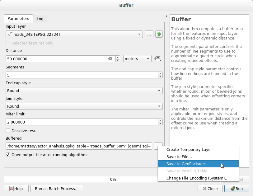
8. Click on Run and then close the Buffer dialog.

이제 여러분의 맵이 다음처럼 보일 것입니다.

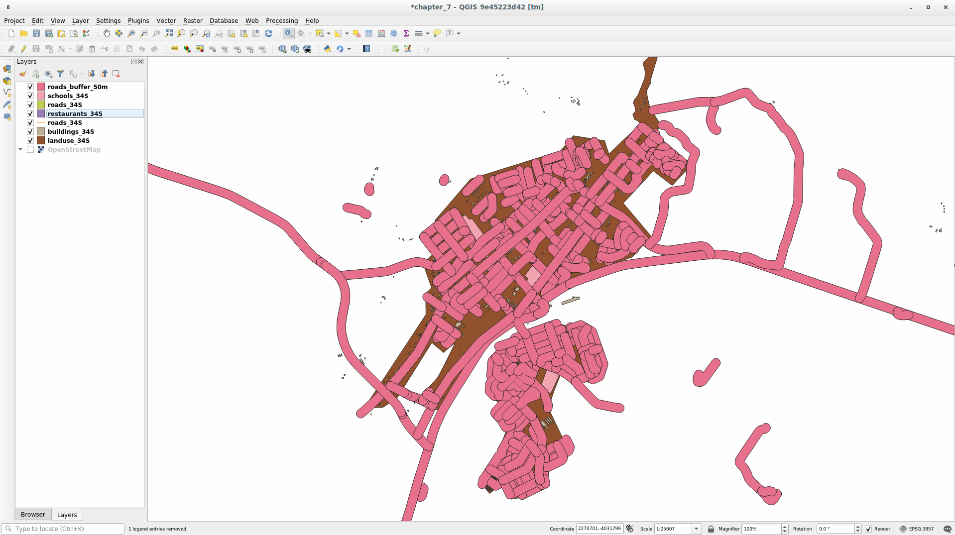
If your new layer is at the top of the Layers list, it will probably obscure much of your map, but this gives you all the areas in your region which are within 50m of a road.

However, you’ll notice that there are distinct areas within your buffer, which correspond to all the individual roads. To get rid of this problem:

1. Uncheck the roads_buffer_50m layer and re-create the buffer using the settings shown here:

   

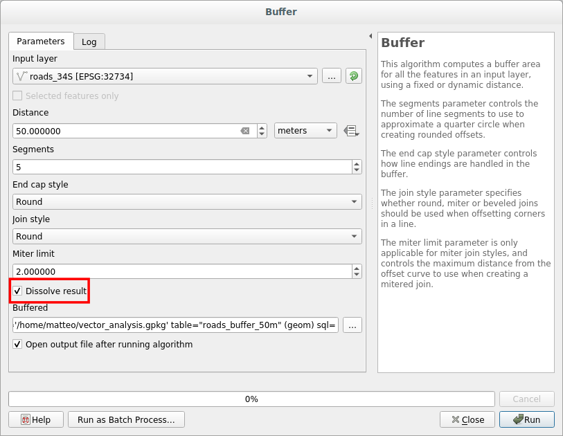
   Note that we’re now checking the Dissolve result box

2. Save the output as roads_buffer_50m_dissolved

3. Click Run and close the Buffer dialog again

Once you’ve added the layer to the Layers panel, it will look like this:

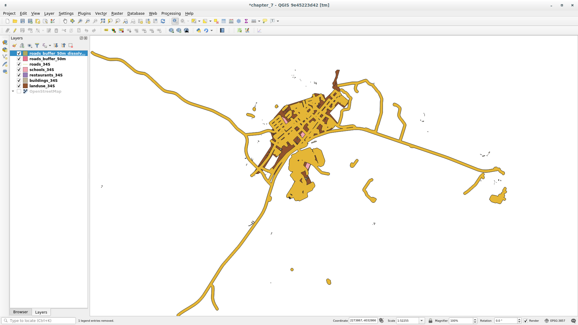
이제 필요 없는 부분들이 사라졌습니다.

참고

The Short Help on the right side of the dialog explains how the algorithm works. If you need more information, just click on the Help button in the bottom part to open a more detailed guide of the algorithm.

7.2.7. Try Yourself 학교로부터의 거리

앞 단계와 동일한 방법으로 학교를 중심으로 하는 버퍼를 생성하십시오.

It needs to be 1 km in radius. Save the new layer in the vector_analysis.gpkg file as schools_buffer_1km_dissolved.

결과 확인

7.2.8. Follow Along: 겹치는 구역

Now we have areas where the road is 50 meters away and there’s a school within 1 km (direct line, not by road). But obviously, we only want the areas where both of these criteria are satisfied. To do that, we’ll need to use the Intersect tool. You can find it in Vector Overlay group within Processing ‣ Toolbox.

1. 다음과 같이 설정하십시오.

   

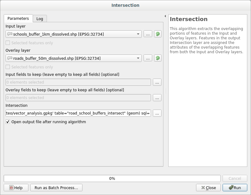
   • The input layers are the two buffers

   • The saving location is, once again, the vector_analysis.gpkg GeoPackage

   • And the output layer name is road_school_buffers_intersect

2. Click Run.

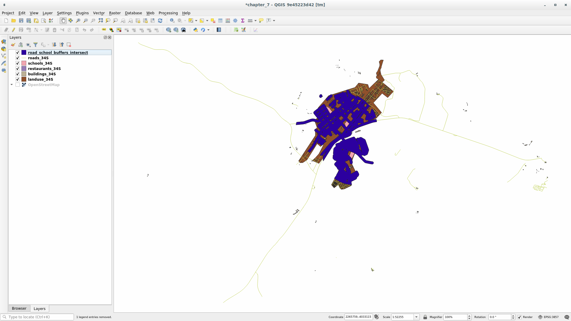
   다음 이미지에서 두 가지 거리 기준을 모두 만족시키는 파란색 구역을 볼 수 있습니다!

   

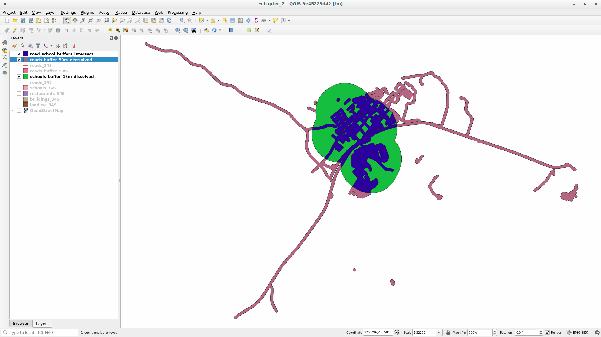
3. 이제 두 버퍼 레이어를 제거하고 겹치는 구역만 보여주는 레이어만 남겨도 됩니다. 원래 그 레이어만을 원했기 때문입니다.

   

7.2.9. Follow Along: Extract the Buildings

Now you’ve got the area that the buildings must overlap. Next, you want to extract the buildings in that area.

1. Look for the menu entry Vector Selection ‣ Extract by location within Processing ‣ Toolbox

2. Set up the algorithm dialog like in the following picture

   

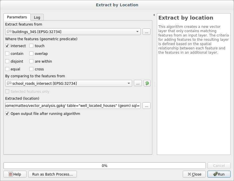
3. Click Run and then close the dialog

4. You’ll probably find that not much seems to have changed. If so, move the well_located_houses layer to the top of the layers list, then zoom in.

   

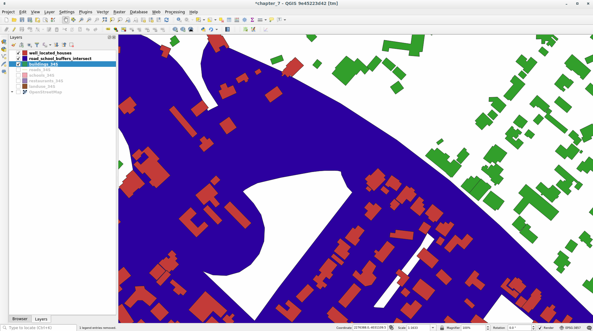
   The red buildings are those which match our criteria, while the buildings in green are those which do not.

5. Now you have two separated layers and can remove buildings_34S from layer list.

7.2.10. Try Yourself 한 번 더 건물을 필터링

이제 학교에서 1km, 도로에서 50m 이내에 있는 모든 건물들을 보여주는 레이어가 생성됐습니다. 다음으로 이 레이어에서 식당으로부터 500m 이내에 있는 건물들만 추려내야 합니다.

Using the processes described above, create a new layer called houses_restaurants_500m which further filters your well_located_houses layer to show only those which are within 500m of a restaurant.

결과 확인

7.2.11. Follow Along: 면적 기준을 만족하는 건물 선택

To see which buildings are of the correct size (more than 100 square meters), we first need to calculate their size.

1. Select the houses_restaurants_500m layer and open the Field Calculator by clicking on the button in the main toolbar or within the attribute table

2. Set it up like this

   

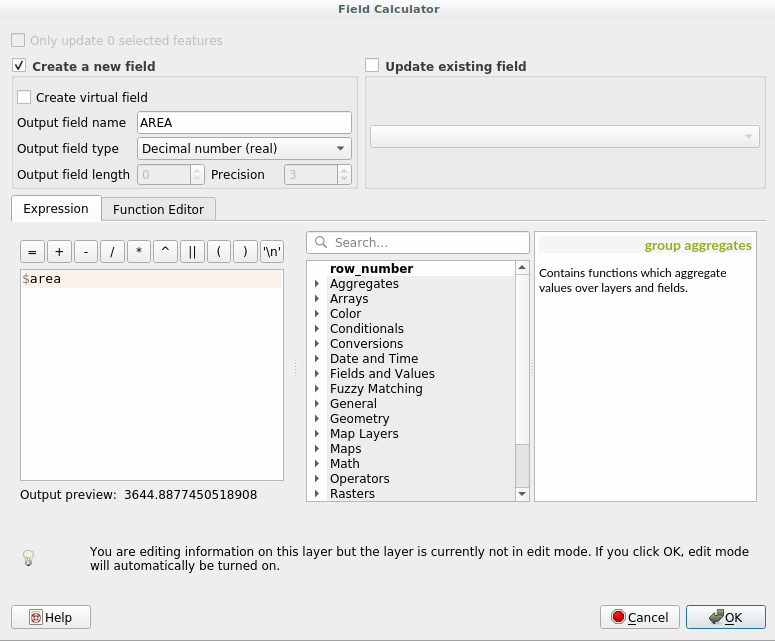
   We are creating the new field AREA that will contain the area of each building square meters.

3. Click OK. The AREA field has been added at the end of the attribute table.

4. 편집 모드 버튼을 한 번 더 클릭해서 편집을 끝내고, 편집 내용을 저장하십시오.

5. Build a query as earlier in this lesson

   

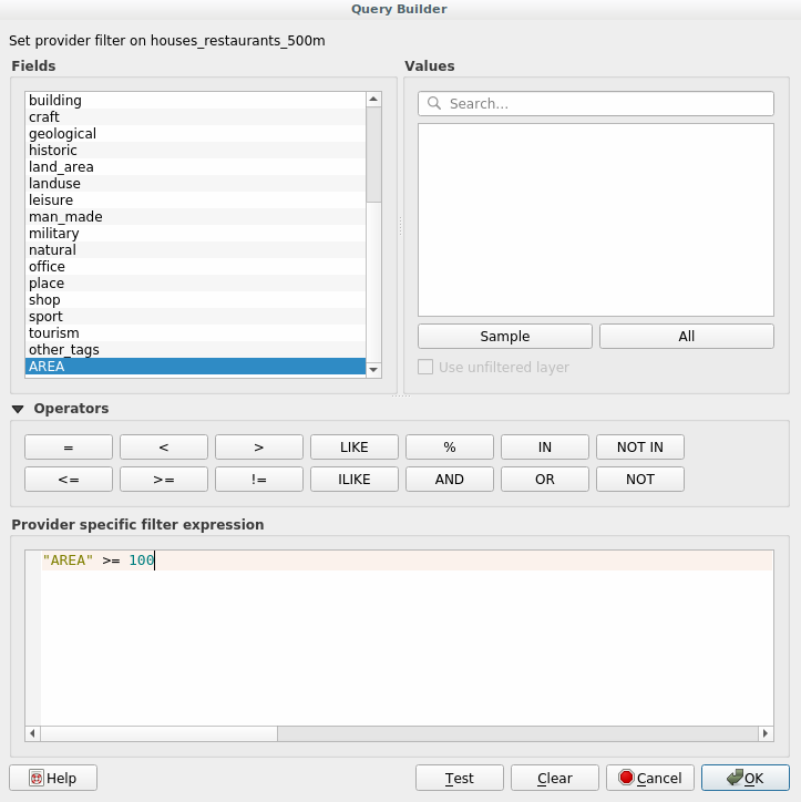
6. OK 를 클릭합니다.

Your map should now only show you those buildings which match our starting criteria and which are more than 100m squared in size.

7.2.12. Try Yourself

Save your solution as a new layer, using the approach you learned above for doing so. The file should be saved within the same GeoPackage database, with the name solution.

7.2.13. In Conclusion

QGIS 벡터 분석 도구와 함께 GIS 문제 해결 접근법을 이용하면, 복합적인 기준을 가진 문제를 쉽고 빠르게 해결할 수 있습니다.

7.2.14. What’s Next?

다음 강의에서는 한 지점에서 다른 지점까지의 최단 거리를 도로를 따라 계산하는 방법을 배워보겠습니다.