8.3. Lesson: Analyse de terrain

Certains types de raster vous permettent de gagner plus de perspicacité dans le terrain que ce qu’ils représentent. Les Modèles Numériques d’Élévation (MNE) sont particulièrement utiles dans ce sens. Dans cette leçon, vous utiliserez les outils d’analyse de terrain pour en savoir plus sur la zone d’étude pour le développement résidentiel proposé plus tôt.

Objectif de cette leçon : Utiliser les outils d’analyse de terrain pour avoir plus d’information sur le terrain.

8.3.1. Follow Along: Calcul d’un Ombrage

We are going to use the same DEM layer as in the previous lesson. If you are starting this chapter from scratch use the Browser panel and load the raster/SRTM/srtm_41_19.tif.

The DEM layer shows you the elevation of the terrain, but it can sometimes seem a little abstract. It contains all the 3D information about the terrain that you need, but it doesn’t look like a 3D object. To get a better look at the terrain, it is possible to calculate a hillshade, which is a raster that maps the terrain using light and shadow to create a 3D-looking image.

We are going to use algorithms of Raster ‣ Raster terrain analysis menu.

1. Click on the Hillshade menu

2. The algorithm allows you to specify where the position of the light source: the Azimuth parameter has values from 0 (North) through 90 (East), 180 (South) and 270 (West) while the Vertical angle sets how high the light is. We will leave the default values:

   

3. Save the file in a new folder raster_analysis within the folder exercise_data with the name hillshade

4. Pour finir, cliquez sur Exécuter

Vous aurez maintenant une nouvelle couche appelée hillshade qui ressemble à cela :

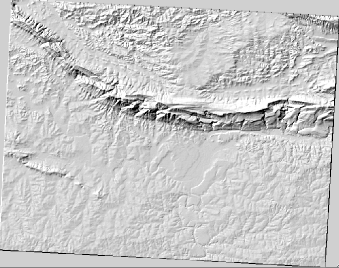
Le résultat semble sympathique et en 3D. Mais pouvons-nous l’améliorer ? L’ombrage semble un peut en plâtre. Pouvons-nous le combiner avec nos autres rasters plus colorés ? C’est effectivement possible en utilisant l’ombrage en tant que couverture.

8.3.2. Follow Along: Utilisation d’un ombrage comme une couverture

Un ombrage peut fournir des informations très utiles sur la lumière du soleil à un moment donné de la journée. Mais il peut aussi être utilisé à des fins esthétiques, pour donner à la carte une meilleure apparence. La clé pour cela est de configurer l’ombrage pour qu’il soit presque complètement transparent.

1. Change the symbology of the original srtm_41_19 layer to use the Pseudocolor scheme as in the previous exercise

2. Hide all the layers except the srtm_41_19 and hillshade layers

3. Click and drag the srtm_41_19 to be beneath the hillshade layer in the Layers panel

4. Set the hillshade layer to be transparent by clicking on the Transparency tab in the layer properties

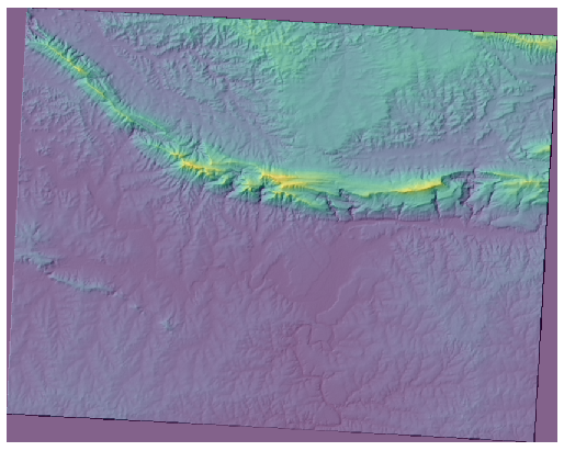
5. Définissez l” Opacité globale à 50%.

   Vous obtiendrez le résultat suivant :

   

6. Switch the hillshade layer off and back on in the Layers panel to see the difference it makes.

En utilisant un ombrage de cette façon, il est possible d’améliorer la topographie du paysage. Si l’effet ne vous semble pas suffisamment fort, vous pouvez changer la transparence de la couche hillshade ; mais bien sûr que plus l’ombrage devient brillant, plus les couleurs derrière lui seront sombres. Vous devrez trouver un équilibre qui fonctionne pour vous.

Remember to save the project when you are done.

8.3.3. Follow Along: Calcul d’une Pente

Une autre chose utile à savoir à propos du terrain est comment est sa pente. Si, par exemple, vous voulez construire des maisons ici, alors vous avez besoin d’un terrain relativement plat.

To do this, you need to use the Slope algorithm of the Processing ‣ Raster terrain analysis.

1. Open the algorithm

2. Choose srtm_41_19 as the Elevation layer

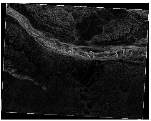
3. Save the output as a file with the name slope in the same folder as the hillshade

4. Click on Run

Now you’ll see the slope of the terrain, with black pixels being flat terrain and white pixels, steep terrain:

8.3.4. Try Yourself Calculating the aspect

Aspect is the compass direction that the slope of the terrain faces. An aspect of 0 means that the slope is North-facing, 90 East-facing, 180 South-facing, and 270 West-facing.

Since this study is taking place in the Southern Hemisphere, properties should ideally be built on a north-facing slope so that they can remain in the sunlight.

Use the Aspect algorithm of the Processing ‣ Raster terrain analysis to get the layer.

Vérifiez vos résultats

8.3.5. Follow Along: Utilisation de la Calculatrice Raster

Rappelez-vous le problème de l’agent immobilier que nous nous sommes posés dans la leçon Analyse Vectorielle. Imaginons que les acheteurs souhaitent maintenant acheter un immeuble et construire un plus petit cottage sur la propriété. Dans l’Hémisphère Sud, nous savons qu’une parcelle idéale pour le développement a besoin d’avoir des zones orientées vers le Nord, et avec une pente de moins de cinq degrés. Mais si la pente est inférieure à 2 degrés, alors l’aspect ne fonctionnera pas.

Heureusement, vous avez déjà des rasters qui vous montrent la pente aussi bien que l’aspect, mais vous n’avez aucune façon de savoir où les deux conditions sont immédiatement satisfaites. Comment cette analyse peut-elle être faite ?

La réponse réside dans la Calculatrice Raster.

QGIS has different raster calculators available:

• Raster ‣ Raster Calculator

• Processing ‣ Raster Analysis ‣ Raster calculator

• Processing ‣ GDAL ‣ Raster miscellaneous ‣ Raster calculator

• SAGA ‣ Raster calculus ‣ Raster calculator

Each tool is leading to the same results, but the syntax may be slightly different and the availability of operators may vary.

We will use Processing ‣ Raster Analysis ‣ Raster calculator.

1. Open the tool by double clicking on it.

   • The upper left part of the dialog lists all the raster layers loaded in the legend as name@N where name is the name of the layer and N is the raster band used.

   • In the upper right part you will see a lot of different operators: stop for a moment to think that a raster is an image, you should see it as a 2D matrix filled with numbers.

2. North is at 0 (zero) degrees, so for the terrain to face north, its aspect needs to be greater than 270 degrees and less than 90 degrees. Therefore the formula is:

   aspect@1 <= 90 OR aspect@1 >= 270
   

3. You have now to set up the raster details, like the cell size, extent and CRS. This can be done manually by filling or it can be automatically set by choosing a Reference layer. Choose this last option by clicking on the … button next to the Reference layer(s) parameter.

4. In the dialog, choose the aspect layer because we want to obtain a layer with the same resolution.

5. Save the layer as aspect_north.

   The dialog should look like:

   

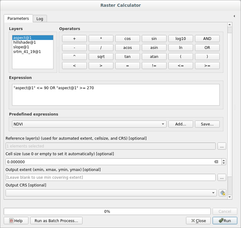
6. Finally click on Run.

Votre résultat doit être cela :

The output values are 0 or 1. What does it mean? The formula we wrote contains the conditional operator OR: therefore the final result will be False (0) and True (1).

8.3.6. Try Yourself More slopes

Maintenant que vous avez fait l’aspect, créez deux nouvelles analyses séparées pour la couche MNE.

• The first will be to identify all areas where the slope is less than or equal to 2 degrees.

• The second is similar, but the slope should be less than or equal to 5 degrees.

• Save them under exercise_data/raster_analysis as slope_lte2.tif and slope_lte5.tif.

Vérifiez vos résultats

8.3.7. Follow Along: Combinaison des résultats de l’analyse raster

Vous avez maintenant trois nouvelles analyses raster sur la couche MNE :

• guilabel:aspect_north : le terrain face au nord

• slope_lte2 : la pente inférieure ou égale à 2 degrés

• slope_lte5 : la pente inférieure ou égale à 5 degrés

Where the conditions of these layers are met, they are equal to 1. Elsewhere, they are equal to 0. Therefore, if you multiply one of these rasters by another one, you will get the areas where both of them are equal to 1.

Les conditions à remplir sont : égal ou inférieur à 5 degrés de pente, le terrain doit être orienté au Nord ; mais égal ou inférieur à 2 degrés de pente, la direction vers laquelle le terrain est orienté n’a pas d’importance.

Therefore, you need to find areas where the slope is at or below 5 degrees AND the terrain is facing north, OR the slope is at or below 2 degrees. Such terrain would be suitable for development.

Pour calculer les zones qui satisfont ces critères :

1. Open your Raster calculator again

2. Use the Layer panel, the Operators buttons, and your keyboard to build this expression in the Expressions text area:

   ( aspect_north@1 = 1 AND slope_lte5@1 = 1 ) OR slope_lte2@1 = 1
   

3. Set the Reference layer(s) parameter as the aspect_north (it does not matter if you choose another one given that all the layers have been calculated from srtm_41_19)

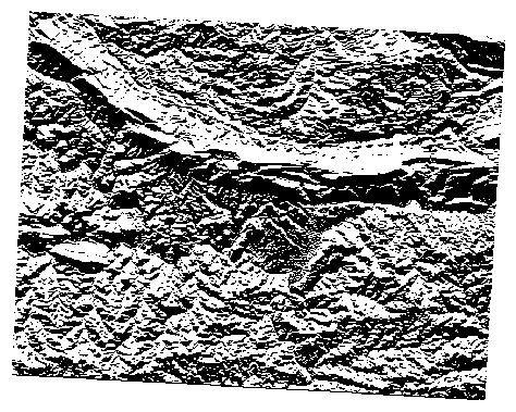
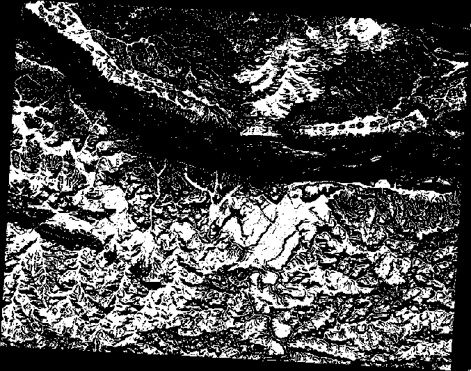
4. Save the output under exercise_data/raster_analysis/ as all_conditions.tif

5. Cliquez sur Exécuter

Vos résultats :

8.3.8. Follow Along: Simplification du Raster

Comme vous pouvez le voir dans l’image du bas, l’analyse combinée nous a laissé avec beaucoup de très petites zones où les conditions sont remplies. Mais elles ne sont pas très utiles pour nos analyses, puisqu’elles sont trop petites pour y construire quelque chose. Éliminons toutes ces toutes petites zones inutiles.

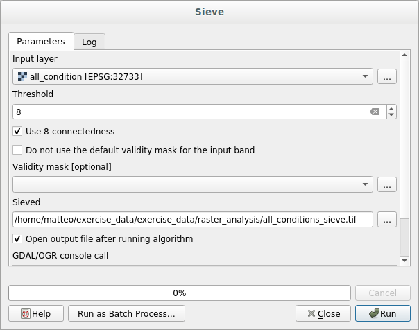
1. Open the Sieve tool Processing ‣ GDAL ‣ Raster Analysis

2. Set the Input file to all_conditions, and the Sieved to all_conditions_sieve.tif (under exercise_data/raster_analysis/).

3. Set both the Threshold to 8 and check Use 8-connectedness.

   

   Once processing is done, the new layer will load into the canvas.

   

   Que se passe-t-il ? La réponse réside dans les fichiers de métadonnées du nouveau raster.

4. View the metadata under the Information tab of the Layer Properties dialog. Look the STATISTICS_MINIMUM value: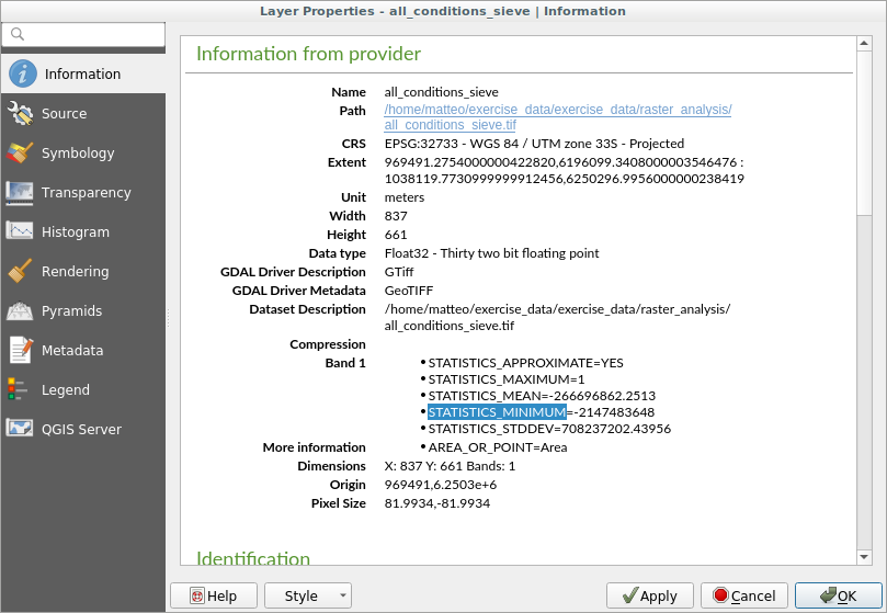

   

   Whereas this raster, like the one it’s derived from, should only feature the values 1 and 0 while it has also a very large negative number. Investigation of the data shows that this number acts as a null value. Since we’re only after areas that weren’t filtered out, let’s set these null values to zero.

5. Open the Raster Calculator again, and build this expression:

   (all_conditions_sieve@1 <= 0) = 0
   

   This will maintain all existing zero values, while also setting the negative numbers to zero; which will leave all the areas with value 1 intact.

6. Save the output under exercise_data/raster_analysis/ as all_conditions_simple.tif.

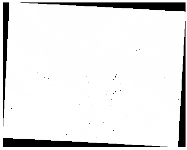
Votre sortie ressemble à cela :

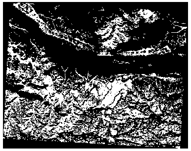
C’est ce qui était attendu : une version simplifiée des résultats précédents. Souvenez-vous que si les résultats que vous obtenez à partir d’un outil ne sont pas ceux que vous attendiez, visualiser les métadonnées (et les attributs vectoriels, si applicable) peut s’avérer essentiel pour résoudre le problème.

8.3.9. Follow Along: Reclassifying the Raster

We use the Raster calculator tool to make some calculation on raster layer. There is another powerful tool that we can use to better extract information from existing layers.

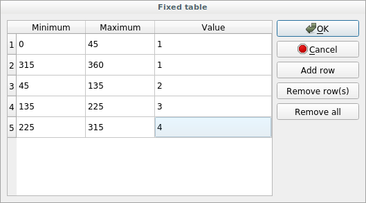
Back to the aspect layer: we know now that it has numeric values within a range from 0 through 360. What we want to do is to reclassify this layer with other discrete values (from 1 to 4) depending on the aspect:

• 1 = North (from 0 to 45 and from 315 to 360);

• 2 = East (from 45 to 135)

• 3 = South (from 135 to 225)

• 4 = West (from 225 to 315)

This operation could be achieved with the raster calculator but the formula would become very very large.

The alternative tool is the Reclassify by table tool within Processing ‣ Raster analysis.

1. Lancez l’outil

2. Choose aspect as the Input raster layer

3. Click on the … of the Reclassification table parameter. A table like dialog will pop up where you can choose the minimum, maximum and new values for each class.

4. Click on the Add row button and add 5 rows. Fill each row as the following picture and click OK:

   

   The method used by the algorithm to treat the threshold values of each class is defined by the Range boundaries parameter.

5. Save the layer as reclassified in the exercise_data/raster_analysis/ folder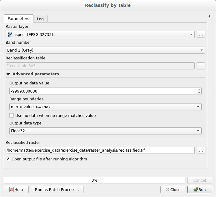

   

6. Click on Run

If you compare the native aspect layer with the reclassified one, there are not big differences. But giving a look at the legend you can see that the values go from 1 to 4.

Let’s give this layer a better style.

1. Open the Layer Styling panel

2. Choose Paletted/Unique values instead of Singleband gray

3. Click on the Classify button to automatically fetch the values and assign them random colors:

   

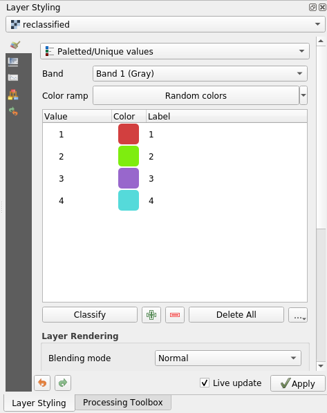
The output should look like this (you can have different colors given that they have been randomly generated):

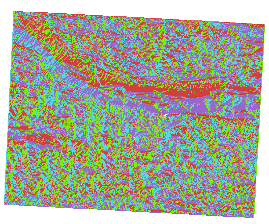
With this reclassification and the paletted style applied to the layer you can immediately see the aspect areas. Cool isn’t it?!

8.3.10. Follow Along: Querying the raster

Unlike vectors, raster layers don’t have an attribute table: each pixel contains one or more numerical values, depending if the raster is singleband or multiband.

All the raster layers we used in this exercise are made by just a single band: depending on the layer, pixel numbers will represent elevation, aspect or slope values.

How can we query the raster layer to know the value of a single pixel? We can use the button to extract this information.

1. Select the tool from the upper toolbar

2. Click on a random location of the srtm_41_19 layer. The Identify Results will appear with the value of the band at the clicked location:

   

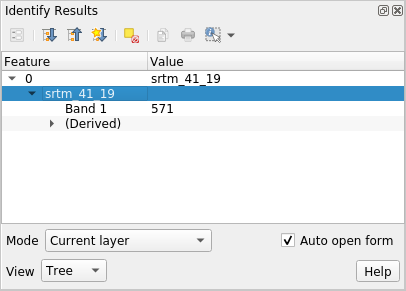
3. You can change the output of the Identify Results panel from the current tree mode to a table one by selecting Table in the View menu at the bottom of the panel:

   

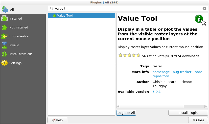
Clicking each pixel to get the value of the raster could become annoying after a while. We can use the Value Tool plugin to solve this problem.

1. Go to Plugins ‣ Manage/Install Plugins…

2. In the All tab, type Value Tool in the search box

3. Select the Value Tool plugin, press Install Plugin and then Close the dialog.

   

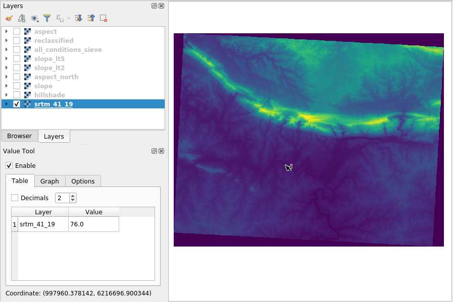
   The new Value Tool panel will appear.

   Astuce

   If you close the panel you can reopen it by enabling it in the View ‣ Panels ‣ Value Tool or by clicking on the new icon of the toolbar.

4. To use the plugin just check the Enable checkbox and be sure that the srtm_41_19 layer is active (checked) in the Layers panel.

5. Move the cursor on the map to immediately know the value of the pixel

   

6. But there is more. The Value Tool plugin allows to query all the active raster layers in the Layers panel. Set the aspect and slope layers active again and hover the mouse on the map:

   

8.3.11. In Conclusion

You’ve seen how to derive all kinds of analysis products from a DEM. These include hillshade, slope and aspect calculations. You’ve also seen how to use the raster calculator to further analyze and combine these results. Finally you learned how to reclassify a layer and how to query the results.

8.3.12. What’s Next?

Maintenant que vous avez deux analyse : l’analyse vectorielle qui vous montre les parcelles susceptibles de convenir, et l’analyse raster qui vont montre le terrain susceptibles de convenir. Comment peut-on les combiner pour arriver à un résultat final pour ce problème ? C’est le sujet de la prochaine leçon, qui commence dans le module suivant.