3.1. Lesson: Travailler avec des données vectorielles
Les données vectorielles sont probablement le type de données que vous rencontrerez le plus souvent dans un usage courant des SIG. Le type vectoriel représente la localisation et la forme des entités géographiques avec des points, des lignes et des polygones (et, pour les données 3D, aussi des surfaces et volumes), tandis que les autres propriétés sont inclues comme attributs (souvent présentées en tableau dans QGIS). On s’en sert d’habitude pour enregistrer des entités discrètes, comme des routes et des groupes de maisons. Les objets d’un jeu de données vectoriel sont appelés entités, et contiennent des données qui décrivent leur localisation et leurs propriétés.
L’objectif de cette leçon : Apprendre à reconnaître la structure des données vectorielles, et la façon de charger des jeux de données vectorielles sur une carte.
3.1.1.  Follow Along: Visualisation des attributs d’une couche
Il est important de comprendre que les données avec lesquelles vous êtes en train de travailler ne montrent pas seulement où ces objets se trouvent dans l’espace, mais aussi vous informent sur ce que sont ces objets.
From the previous exercise, you should have the rivers layer loaded in your map. The lines that you can see right now are merely the position of the rivers: this is the spatial data.
To see all the available data in the rivers layer,
select it in the Layers panel and click the  button.
It will show you a table with more data about the rivers layer. This is the layer’s Attribute table. A row is called a record, and represents a river feature. A column is called a field, and represents a property of the river. Cells show attributes.
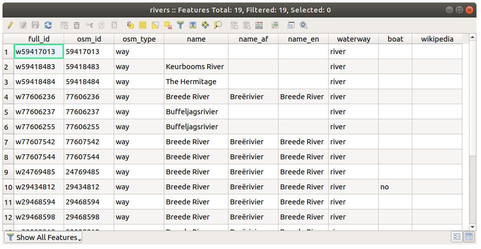
Ces définitions sont communément utilisées dans les SIG, c’est pourquoi il est essentiel de s’en souvenir !
Vous pouvez maintenant fermer la table d’attributs.
3.1.2. Try Yourself Exploring Vector Data Attributes
How many fields are available in the rivers layer?
Tell us a bit about the
townplaces in your dataset.
3.1.3. Follow Along: Loading Vector Data From GeoPackage Database
Databases allow you to store a large volume of associated data in one file. You may already be familiar with a database management system (DBMS) such as Libreoffice Base or MS Access. GIS applications can also make use of databases. GIS-specific DBMSes (such as PostGIS) have extra functions, because they need to handle spatial data.
The GeoPackage open format is a container that
allows you to store GIS data (layers) in a single file.
Unlike the ESRI Shapefile format (e.g. the protected_areas.shp dataset
you loaded earlier), a single GeoPackage file can contain various data (both
vector and raster data) in different coordinate reference systems, as well as
tables without spatial information; all these features allow you to share data
easily and avoid file duplication.
In order to load a layer from a GeoPackage, you will first need to create the connection to it:
Click on the
 Open Data Source Manager button.
On the left click on the
 GeoPackage tab.
Click on the New button and browse to the
training_data.gpkgfile in theexercise_datafolder you downloaded before.Select the file and press Open. The file path is now added to the Geopackage connections list, and appears in the drop-down menu.
You are now ready to add any layer from this GeoPackage to QGIS.
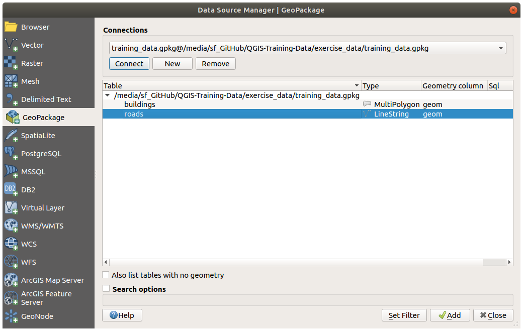
Click on the Connect button. In the central part of the window you should now see the list of all the layers contained in the GeoPackage file.
Select the roads layer and click on the Add button.
A roads layer is added to the Layers panel with features displayed on the map canvas.
Click on Close.
Congratulations! You have loaded the first layer from a GeoPackage.
3.1.4. Follow Along: Loading Vector Data From a SpatiaLite Database with the Browser
QGIS provides access to many other database formats. Like GeoPackage, the SpatiaLite database format is an extension of the SQLite library. And adding a layer from a SpatiaLite provider follows the same rules as described above: Create the connection –> Enable it –> Add the layer(s).
While this is one way to add SpatiaLite data to your map, let’s explore another powerful way to add data: the Browser.
Click the
icon to open the Data Source Manager
window.Click on the
 Browser tab.
In this tab you can see all the storage disks connected to your computer as well as entries for most of the tabs in the left. These allow quick access to connected databases or folders.
For example, click on the drop-down icon next to the
 GeoPackage entry. You’ll see the
 training-data.gpkgfile we previously connected to (and its layers, if expanded).Right-click the
 SpatiaLite entry and select
New Connection….
SpatiaLite entry and select
New Connection….Navigate to the
exercise_datafolder, select thelanduse.sqlitefile and click Open.Notice that a
 landuse.sqlite entry has
been added under the SpatiaLite one.
landuse.sqlite entry has
been added under the SpatiaLite one.Expand the
landuse.sqlite entry.Double-click the
 landuse layer or select and
drag-and-drop it onto the map canvas. A new layer is added to the
Layers panel and its features are displayed on the map canvas.
landuse layer or select and
drag-and-drop it onto the map canvas. A new layer is added to the
Layers panel and its features are displayed on the map canvas.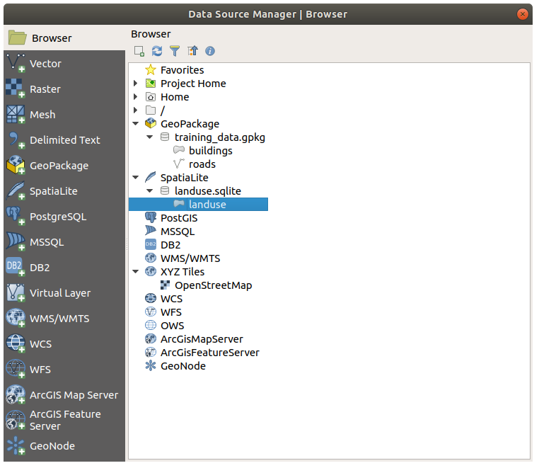
Astuce
Enable the Browser panel in and use it to add your data. It’s a handy shortcut for the tab, with the same functionality.
Note
Remember to save your project frequently! The project file doesn’t contain any of the data itself, but it remembers which layers you loaded into your map.
3.1.5.  Try Yourself Load More Vector Data
Load the following datasets from the exercise_data folder into your map
using any of the methods explained above:
buildings
water
3.1.6. Follow Along: Réorganisation des calques
Les calques dans votre liste de calques sont dessinés sur la carte dans un certain ordre. Le calque en bas de la liste est dessiné en premier, et le calque en haut est dessiné en dernier. En changeant leur ordre dans la liste, vous pouvez changer l’ordre suivant lesquel ils sont dessinés.
Note
You can alter this behavior using the Control rendering order checkbox beneath the Layer Order panel. We will however not discuss this feature yet.
L’ordre dans lequel les couches ont été chargées dans la carte n’est probablement pas logique à ce stade. Il est possible que la couche des routes soit complètement cachée parce que les autres couches sont au-dessus d’elle.
Par exemple, cet ordre de couche…
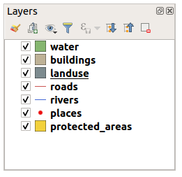
… would result in roads and places being hidden as they run underneath the polygons of the landuse layer.
Pour résoudre le problème :
Cliquez et glissez sur la couche dans la légende de la carte.
Réorganiser-les pour obtenir ça :
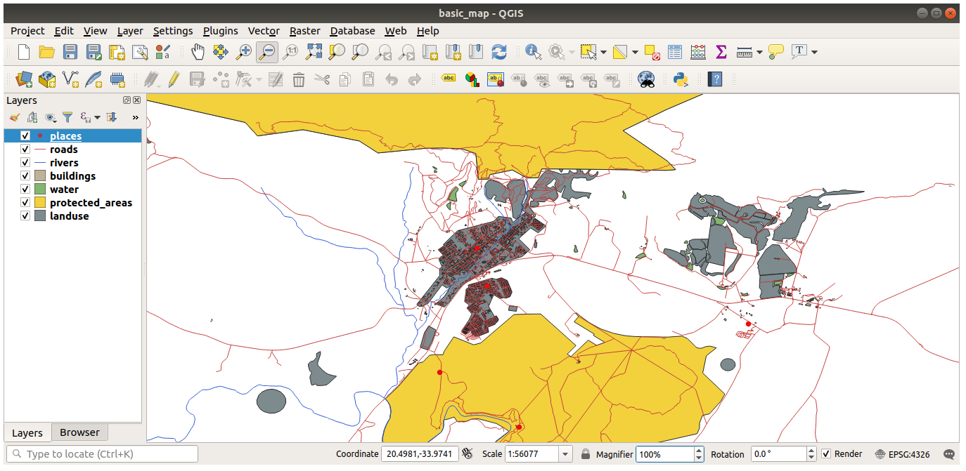
Vous verrez que la carte a maintenant visuellement plus de sens, avec les routes et les bâtiments qui apparaissent au-dessus des régions d’utilisation du sol.
3.1.7. In Conclusion
Maintenant vous avez ajouté tous les calques dont vous aviez besoin à partir de plusieurs différentes sources.
3.1.8. What’s Next?
En utilisant la palette de couleur aléatoire automatiquement assignée lors du chargement des couches, votre carte actuelle n’est sans doute pas facile à lire. Il est donc préférable d’assigner votre propre choix de couleurs et de symboles aux couches. C’est ce que nous verrons dans la prochaine leçon.