Integração GRASS SIG¶

Iniciando o módulo GRASS¶

Para usar as funcionalidades e/ou visualizar camadas vectoriais e raster do GRASS no QGIS, deve seleccionar e carregar o módulo GRASS com o Gestor de Módulos. Portanto, vá ao menu Módulos ‣ Gerir Módulos, e seleccione GRASS e clique [OK].

Pode agora iniciar o carregamento das camadas raster e vectorial a partir de um file:LOCALIZAÇÃO (see section sec_load_grassdata) GRASS. Ou pode criar um novo LOCALIZAÇÃO com o QGIS (veja a secção Criando uma nova LOCALIZAÇÃO GRASS) e importe alguns dados vectoriais e raster (veja a Secção Importando dados para uma LOCALIZAÇÃO GRASS) para mais análises com a Caixa de Ferramentas GRASS (veja a secção The GRASS toolbox).

Carregando as camadas raster e vectoriais GRASS¶

Com o módulo GRASS, pode carregar camadas vectoriais e raster usando o botão apropriadado no menu da barra de ferramentas. Como exemplo, nós usamos o conjunto de dados QGIS do alaska (veja Secção Amostra de Dados). Inclue uma pequena amostra de LOCALIZAÇÃO GRASS com 3 camadas vectoriais e 1 raster de elevação.

1. Crie uma nova pasta grassdata, transfira o conjunto de dados QGIS ‘Alaska’ qgis_sample_data.zip apartir do http://download.osgeo.org/qgis/data/ e descompacte o ficheiro no grassdata.

2. Iniciar o QGIS.

3. Se ainda não fez numa sessão QGIS anterior, carrega o módulo GRASS clicando no Módulos ‣ Gestor de Módulos e active GRASS. A barra de ferramentas GRASS aparece na janela principal do QGIS.

4. Na barra de ferramentas GRASS, clique no ícone ^{Abrir conjunto de mapas} para iniciar o assistente de instalação do CONJUNTO DE DADOS.

5. Para a Gisdbase procure e seleccione ou introduza o directório para a nova pasta criada grassdata.

6. Poderá agora ser capaz de seleccionar a LOCALIZAÇÃO alaska e o guilabel:CONJUNTO DE DADOS demo.

7. Clique [OK]. Repare que algumas das ferramentas na barra de ferramentas GRASS que estão desactivadas agora estão activas.

8. Clique no ^{Adicionar camada raster GRASS}, escolha o nome do mapa gtopo30 e cliquem em [OK]. A camada de elevação irá ser visualizada.

9. Click on ^{Add GRASS vector layer}, choose the map name alaska and click [OK]. The Alaska boundary vector layer will be overlayed on top of the gtopo30 map. You can now adapt the layer properties as described in chapter The Vector Properties Dialog, e.g. change opacity, fill and outline color.

10. Carregue também as outras duas camadas vectoriais rivers e airports e adaptar as suas propriedades.

As you see, it is very simple to load GRASS raster and vector layers in QGIS. See following sections for editing GRASS data and creating a new LOCATION. More sample GRASS LOCATIONs are available at the GRASS website at http://grass.osgeo.org/download/sample-data/.

LOCALIZAÇÃO GRASS e CONJUNTO DE MAPAS¶

GRASS data are stored in a directory referred to as GISDBASE. This directory often called grassdata, must be created before you start working with the GRASS plugin in QGIS. Within this directory, the GRASS GIS data are organized by projects stored in subdirectories called LOCATION. Each LOCATION is defined by its coordinate system, map projection and geographical boundaries. Each LOCATION can have several MAPSETs (subdirectories of the LOCATION) that are used to subdivide the project into different topics, subregions, or as workspaces for individual team members (Neteler & Mitasova 2008 Literatura e Referências Web). In order to analyze vector and raster layers with GRASS modules, you must import them into a GRASS LOCATION (This is not strictly true - with the GRASS modules r.external and v.external you can create read-only links to external GDAL/OGR-supported data sets without importing them. But because this is not the usual way for beginners to work with GRASS, this functionality will not be described here.).

Figure GRASS location 1:

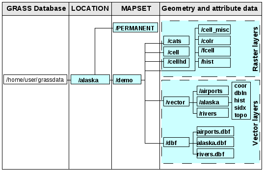
Dados GRASS na LOCALIZAÇÃO alaska

Criando uma nova LOCALIZAÇÃO GRASS¶

O exemplo aqui é como a amostra GRASS LOCALIZAÇÃO alaska, que é projectado na projecção Albers Equal Area com a unidade em pés e que foi criado para a amostra do conjunto de dados QGIS. Esta amostra GRASS LOCALIZAÇÃO alaska irá ser usado para todos os exemplos e exercícios nos seguintes capítulos do GRASS GIS. É útil transferir e instalar o conjunto de dados no computador Amostra de Dados).

1. Inicie o QGIS e certifique-se que o módulo GRASS foi carregado.

2. Visualize a shapefile alaska.shp (veja Secção vector_load_shapefile) a partir do Amostra de Dados do conjunto de dados QGIS alaska.

3. Na barra de ferramentas GRASS, clique no ícone ^{Novo conjunto de mapas} para iniciar o assistente de instalação do CONJUNTO DE DADOS.

4. Seleccione uma pasta de base de dados GRASS (GISDBASE) grassdata ou crie um para a nova LOCALIZAÇÃO usando um gestor de ficheiros no seu computador. De seguida, clique em [Seguinte].

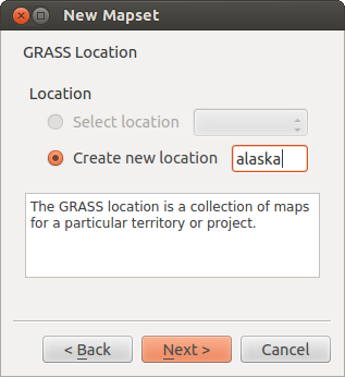
5. Nós podemos usar este assistente para criar um novo CONJUNTO DE MAPAS dentro de uma LOCALIZAÇÃO existente (veja secção Adicionando um novo CONJUNTO DE MAPAS) ou pata criar juntamente um nova LOCALIZAÇÃO. Seleccione Criar nova localização (veja figure_grass_location_2).

6. Introduza o nome para LOCALIZAÇÃO - nós usámos ‘alaska’ e clique [Seguinte].

7. Defina a projecção clicando no botão Projecção para activar a lista de projecção.

8. We are using Albers Equal Area Alaska (feet) projection. Since we happen to know that it is represented by the EPSG ID 2964, we enter it in the search box. (Note: If you want to repeat this process for another LOCATION and projection and haven’t memorized the EPSG ID, click on the ^{CRS Status} icon in the lower right-hand corner of the status bar (see Section Working with Projections)).

9. Em Filtrar insira 2964 para seleccionar a projecção.

10. Clique [Seguinte].

11. Para definir uma região padrão, nós temos de introduzir os limites da LOCALIZAÇÃO na direcção norte, sul, oeste e este. Aqui simplesmente clicamos no botão [Definir a extensão actual do QGIS], para aplicar a extensão da camada carregada alaska.shp como região de extensão padrão do GRASS.

12. Clique [Seguinte].

13. Necessitaremos também de definir o CONJUNTO DE MAPAS dentro da nossa nova LOCALIZAÇÃO. Pode dar o nome que quiser - nós usámos ‘demo’ (quando é criado uma nova LOCALIZAÇÃO). O GRASS cria automaticamente um CONJUNTO DE MAPAS especial denominado de PERMANENTE desenhado para armazenar os dados importantes para o projecto, é uma extensão espacial padrão com definições de sistemas de coordenadas (Neteler & Mitasova 2008 Literatura e Referências Web).

14. Verifique o sumário para ter a certeza que está correcto e clique em [Concluído].

15. A nova LOCALIZAÇÃO ‘alaska’ e dois CONJUNTO DE MAPAS ‘demo’ e ‘PERMANENTE’ são criados. O conjunto de trabalho actualmente aberto é o ‘demo’, como tinha definido.

16. Repare que algumas das ferramentas na barra de ferramentas GRASS que estão desactivadas agora estão activas.

Figure GRASS location 2:

Criando uma nova LOCALIZAÇÃO GRASS ou um novo CONJUNTO DE MAPAS no QGIS

Se achar que são muitos passos, não é assim tão mau e há uma forma rápida para criar uma LOCALIZAÇÃO. A LOCALIZAÇÃO 'alaska não está preparada para importação de dados (veja Secção Importando dados para uma LOCALIZAÇÃO GRASS). Pode também usar os dados vectoriais e raster existentes na amostra GRASS LOCALIZAÇÃO ‘alaska’ incluída no conjunto de dados do QGIS ‘Alaska’ Amostra de Dados e siga para a Secção O modelo de dados vectoriais do GRASS.

Importando dados para uma LOCALIZAÇÃO GRASS¶

This Section gives an example how to import raster and vector data into the ‘alaska’ GRASS LOCATION provided by the QGIS ‘Alaska’ dataset. Therefore we use a landcover raster map landcover.img and a vector GML file lakes.gml from the QGIS ‘Alaska’ dataset Amostra de Dados.

1. Inicie o QGIS e certifique-se que o módulo GRASS foi carregado.

2. Na barra de ferramentas GRASS, clique no ícone ^{Abrir CONJUNTO DE MAPAS} para trazer o assistente de CONJUNTO DE MAPAS.

3. Seleccione como base de dados GRASS a pasta grassdata no conjunto de dados QGIS alasca, assim como LOCALIZAÇÃO ‘alaska’, e o CONJUNTO DE MAPAS ‘demo’ e clique [OK].

4. Agora clique no ícone ^{Abrir ferramentas GRASS}. O diálogo da Caixa de Ferramentas GRASS (veja secção The GRASS toolbox) aparece.

5. To import the raster map landcover.img, click the module r.in.gdal in the Modules Tree tab. This GRASS module allows to import GDAL supported raster files into a GRASS LOCATION. The module dialog for r.in.gdal appears.

6. Procure na pasta raster no conjunto de dados QGIS ‘Alaska’ e seleccione o ficheiro landcover.img.

7. As raster output name define landcover_grass and click [Run]. In the Output tab you see the currently running GRASS command r.in.gdal -o input=/path/to/landcover.img output=landcover_grass.

8. Quando diz Finalizado com sucesso clique em [Ver Saída]. A camada raster landcover:grass está agora importada dentro do GRASS e será visualizada no enquadramento do QGIS.

9. To import the vector GML file lakes.gml, click the module v.in.ogr in the Modules Tree tab. This GRASS module allows to import OGR supported vector files into a GRASS LOCATION. The module dialog for v.in.ogr appears.

10. Procure na pasta por gml no conjunto de dados QGIS Alaska e seleccione o ficheiro lakes.gml como ficheiro OGR.

11. As vector output name define lakes_grass and click [Run]. You don’t have to care about the other options in this example. In the Output tab you see the currently running GRASS command v.in.ogr -o dsn=/path/to/lakes.gml output=lakes\_grass.

12. Quando diz Finalizado com Sucesso clique [Ver Saída]. O ficheiro da camada vectorial lakes_grass foi importado para o GRASS e irá visualizar no enquadramento do QGIS.

O modelo de dados vectoriais do GRASS¶

É importante perceber previamente o modelo de dados vectorial GRASS antes da digitalização.

O GRASS usa um modelo topológico vectorial.

This means that areas are not represented as closed polygons, but by one or more boundaries. A boundary between two adjacent areas is digitized only once, and it is shared by both areas. Boundaries must be connected and closed without gaps. An area is identified (and labeled) by the centroid of the area.

Besides boundaries and centroids, a vector map can also contain points and lines. All these geometry elements can be mixed in one vector and will be represented in different so called ‘layers’ inside one GRASS vector map. So in GRASS a layer is not a vector or raster map but a level inside a vector layer. This is important to distinguish carefully (Although it is possible to mix geometry elements, it is unusual and even in GRASS only used in special cases such as vector network analysis. Normally you should prefere to store different geometry elements in different layers.).

It is possible to store several ‘layers’ in one vector dataset. For example, fields, forests and lakes can be stored in one vector. Adjacent forest and lake can share the same boundary, but they have separate attribute tables. It is also possible to attach attributes to boundaries. For example, the boundary between lake and forest is a road, so it can have a different attribute table.

The ‘layer’ of the feature is defined by ‘layer’ inside GRASS. ‘Layer’ is the number which defines if there are more than one layer inside the dataset, e.g. if the geometry is forest or lake. For now, it can be only a number, in the future GRASS will also support names as fields in the user interface.

Attributes can be stored inside the GRASS LOCATION as DBase or SQLITE3 or in external database tables, for example PostgreSQL, MySQL, Oracle, etc.

Os atributos nas tabelas das base de dados estão ligados aos elementos de geometria usando o valor ‘categoria’.

‘Categoria’ (chave, ID) é um inteiro anexado às primitivas da geometria, e é usado como ligação a uma coluna de chave na tabela da base de dados.

Criando uma nova camada vectorial GRASS¶

To create a new GRASS vector layer with the GRASS plugin click the ^{Create new GRASS vector} toolbar icon. Enter a name in the text box and you can start digitizing point, line or polygon geometries, following the procedure described in Section Digitalizando e editando as camadas vectoriais GRASS.

In GRASS it is possible to organize all sort of geometry types (point, line and area) in one layer, because GRASS uses a topological vector model, so you don’t need to select the geometry type when creating a new GRASS vector. This is different from Shapefile creation with QGIS, because Shapefiles use the Simple Feature vector model (see Section Criando novas camadas Vectoriais).

Digitalizando e editando as camadas vectoriais GRASS¶

The digitizing tools for GRASS vector layers are accessed using the ^{Edit GRASS vector layer} icon on the toolbar. Make sure you have loaded a GRASS vector and it is the selected layer in the legend before clicking on the edit tool. Figure figure_grass_digitizing_2 shows the GRASS edit dialog that is displayed when you click on the edit tool. The tools and settings are discussed in the following sections.

Barra de Ferramentas

In figure_grass_digitizing_1 you see the GRASS digitizing toolbar icons provided by the GRASS plugin. Table table_grass_digitizing_1 explains the available functionalities.

Figure GRASS digitizing 1:

Barra de Ferramentas Digitalização GRASS

Ícone	Ferramenta	Finalidade
	Novo Ponto	Digitalizar um novo ponto
	Nova Linha	Digitalizar nova linha
	Novo Limite	Digitalizar novo limite (finalizar seleccionando uma nova ferramenta)
	Novo Centróide	Digitalizar um novo centróide (rótulo com a área existente)
	Mover vértice	Mover um vértice de uma linha existente ou limite e identificar nova posição
	Adicionar vértice	Adicionar um novo vértice a uma linha existente
	Apagar vértice	Apagar vértice de uma linha existente (confirme o vértice seleccionado clicando com outro clique)
	Mover elemento	Mover o limite seleccionado, linha, ponto ou centróide e clique na nova posição
	Dividir linha	Dividir uma linha existente em 2 partes
	Apagar elemento	Delete existing boundary, line, point or centroid (confirm selected element by another click)
	Editar atributos	Editar os atributos do elemento seleccionado (note que um elemento pode representar mais elementos, veja acima)
	Fechar	Feche a sessão e guarde o estado actual (reconstrução da topologia depois)

Tabela GRASS Digitalização 1: Ferramentas de Digitalização GRASS

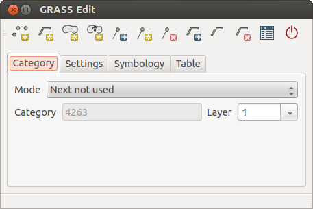
Separador Categoria

O separador Categoria permite definir a forma de como os valores categoria serão atribuídos a um novo elemento de geometria.

Figure GRASS digitizing 2:

Separador de Digitalização de Categorias

• Modo: que valor de categoria deverá ser aplicado aos novos elementos de geometria.

  • Next not used - apply next not yet used category value to geometry element.

  • Entrada manual - defina manualmente os valores de categoria para o elemento da geometria no campo de entrada -‘Categoria’.

  • Sem categoria - Não aplica o valor da categoria ao elemento de geometria. Isto é por exemplo, usado para limites de áreas, porque os valores da categoria são ligados através do centróide.

• Categoria - Um número (ID) é anexado a cada elemento de geometria digitalizado. É usado para ligar cada elemento de geometria com os seus atributos.

• Campo(camada) - Cada elemento de geometria pode ser ligada a várias tabelas de atributos usando diferentes camadas de geometria GRASS. O número da camada padrão é 1.

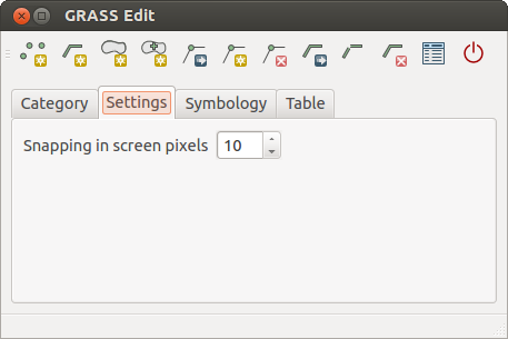
Separador das Configurações

The Settings tab allows you to set the snapping in screen pixels. The threshold defines at what distance new points or line ends are snapped to existing nodes. This helps to prevent gaps or dangles between boundaries. The default is set to 10 pixels.

Figure GRASS digitizing 3:

Separador de Configurações de Digitalização GRASS

Separador da Simbologia

The Symbology tab allows you to view and set symbology and color settings for various geometry types and their topological status (e.g. closed / opened boundary).

Figure GRASS digitizing 4:

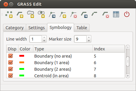
GRASS Digitizing Symbolog Tab

Separador Tabela

The Table tab provides information about the database table for a given ‘layer’. Here you can add new columns to an existing attribute table, or create a new database table for a new GRASS vector layer (see Section Criando uma nova camada vectorial GRASS).

Figure GRASS digitizing 5:

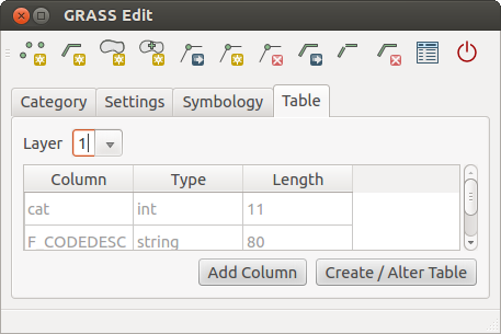
GRASS Digitizing Table Tab

A ferramenta da região GRASS¶

The region definition (setting a spatial working window) in GRASS is important for working with raster layers. Vector analysis is by default not limited to any defined region definitions. But all newly-created rasters will have the spatial extension and resolution of the currently defined GRASS region, regardless of their original extension and resolution. The current GRASS region is stored in the $LOCATION/$MAPSET/WIND file, and it defines north, south, east and west bounds, number of columns and rows, horizontal and vertical spatial resolution.

It is possible to switch on/off the visualization of the GRASS region in the QGIS canvas using the ^{Display current GRASS region} button.

With the ^{Edit current GRASS region} icon you can open a dialog to change the current region and the symbology of the GRASS region rectangle in the QGIS canvas. Type in the new region bounds and resolution and click [OK]. It also allows to select a new region interactively with your mouse on the QGIS canvas. Therefore click with the left mouse button in the QGIS canvas, open a rectangle, close it using the left mouse button again and click [OK].

The GRASS module g.region provide a lot more parameters to define an appropriate region extend and resolution for your raster analysis. You can use these parameters with the GRASS Toolbox, described in Section The GRASS toolbox.

The GRASS toolbox¶

The ^{Open GRASS Tools} box provides GRASS module functionalities to work with data inside a selected GRASS LOCATION and MAPSET. To use the GRASS toolbox you need to open a LOCATION and MAPSET where you have write-permission (usually granted, if you created the MAPSET). This is necessary, because new raster or vector layers created during analysis need to be written to the currently selected LOCATION and MAPSET.

Figure GRASS toolbox 1:

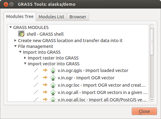
Árvore de Módulos e Caixa de Ferramentas GRASS

The GRASS Shell inside the GRASS Toolbox provides access to almost all (more than 330) GRASS modules through a command line interface. To offer a more user friendly working environment, about 200 of the available GRASS modules and functionalities are also provided by graphical dialogs within the GRASS plugin Toolbox.

Trabalhando com os módulos do GRASS¶

The GRASS Shell inside the GRASS Toolbox provides access to almost all (more than 300) GRASS modules in a command line interface. To offer a more user friendly working environment, about 200 of the available GRASS modules and functionalities are also provided by graphical dialogs.

A complete list of GRASS modules available in the graphical Toolbox in QGIS version 2.0 is available in the GRASS wiki (http://grass.osgeo.org/wiki/GRASS-QGIS_relevant_module_list).

It is also possible to customize the GRASS Toolbox content. This procedure is described in Section Customizing the GRASS Toolbox.

As shown in figure_grass_toolbox_1 , you can look for the appropriate GRASS module using the thematically grouped Modules Tree or the searchable Modules List tab.

Clicando no ícone do módulo gráfico será adicionado um novo separador ao diálogo da caixa de ferramentas fornecendo novos sub-separadores Opções, Saída e Manual.

Opções

The Options tab provides a simplified module dialog where you can usually select a raster or vector layer visualized in the QGIS canvas and enter further module specific parameters to run the module.

Figure GRASS module 1:

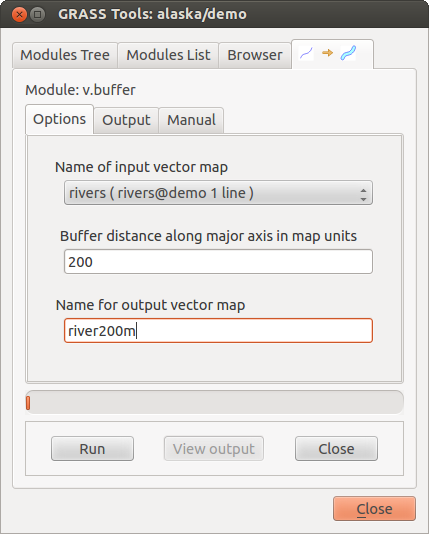
Opções dos Módulos da Caixa de Ferramentas do GRASS

The provided module parameters are often not complete to keep the dialog clear. If you want to use further module parameters and flags, you need to start the GRASS Shell and run the module in the command line.

A new feature since QGIS 1.8 is the support for a show advanced options button below the simplified module dialog in the Options tab. At the moment it is only added to the module v.in.ascii as an example use, but will probably be part of more / all modules in the GRASS toolbox in future versions of QGIS. This allows to use the complete GRASS module options without the need to switch to the GRASS Shell.

Ficheiro de Saída

Figure GRASS module 2:

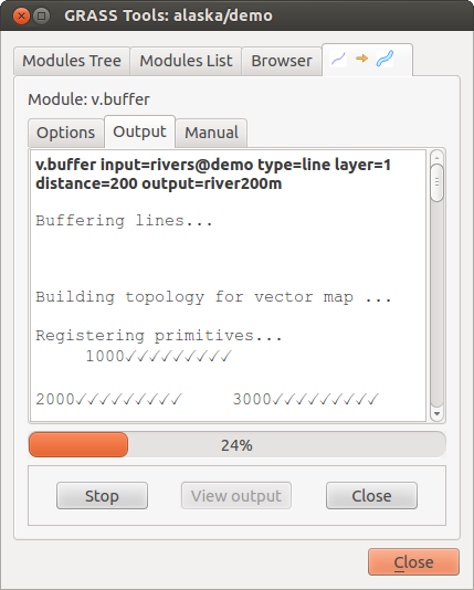
GRASS Toolbox Module Output

The Output tab provides information about the output status of the module. When you click the [Run] button, the module switches to the Output tab and you see information about the analysis process. If all works well, you will finally see a Successfully finished message.

Manual

Figure GRASS module 3:

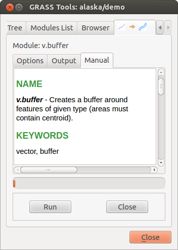
GRASS Toolbox Module Manual

The Manual tab shows the HTML help page of the GRASS module. You can use it to check further module parameters and flags or to get a deeper knowledge about the purpose of the module. At the end of each module manual page you see further links to the Main Help index, the Thematic index and the Full index. These links provide the same information as if you use the module g.manual.

Tip

Exibir os resultados imediatamente

Se quiser exibir os seus resultados do cálculo imediatamente no seu enquadramento do mapa, pode usar o botão ‘Ver ficheiro de saída’ no fundo do separador do módulo.

Exemplos de módulos GRASS¶

Os seguintes exemplos irão demonstrar o poder de alguns módulos GRASS.

Criando linhas de contorno¶

The first example creates a vector contour map from an elevation raster (DEM). Assuming you have the Alaska LOCATION set up as explained in Section Importando dados para uma LOCALIZAÇÃO GRASS.

• First open the location by clicking the ^{Open mapset} button and choosing the Alaska location.
• Now load the gtopo30 elevation raster by clicking ^{Add GRASS raster layer} and selecting the gtopo30 raster from the demo location.
• Now open the Toolbox with the ^{Open GRASS tools} button.
• In the list of tool categories double click Raster ‣ Surface Management ‣ Generate vector contour lines.
• Now a single click on the tool r.contour will open the tool dialog as explained above Trabalhando com os módulos do GRASS. The gtopo30 raster should appear as the Name of input raster.
• Type into the Increment between Contour levels the value 100. (This will create contour lines at intervals of 100 meters.)
• Type into the Name for output vector map the name ctour_100.
• Click [Run] to start the process. Wait for several moments until the message Successfully finished appears in the output window. Then click [View Output] and [Close].

Since this is a large region, it will take a while to display. After it finishes rendering, you can open the layer properties window to change the line color so that the contours appear clearly over the elevation raster, as in The Vector Properties Dialog.

Next zoom in to a small mountainous area in the center of Alaska. Zooming in close you will notice that the contours have sharp corners. GRASS offers the v.generalize tool to slightly alter vector maps while keeping their overall shape. The tool uses several different algorithms with different purposes. Some of the algorithms (i.e. Douglas Peuker and Vertex reduction) simplify the line by removing some of the vertices. The resulting vector will load faster. This process will be used when you have a highly detailed vector, but you are creating a very small scale map, so the detail is unnecessary.

Tip

**A ferramenta de simplificação

Note that the QGIS fTools plugin has a Simplify geometries ‣ tool that works just like the GRASS v.generalize Douglas-Peuker algorithm.

However, the purpose of this example is different. The contour lines created by r.contour have sharp angles that should be smoothed. Among the v.generalize algorithms there is Chaikens which does just that (also Hermite splines). Be aware that these algorithms can add additional vertices to the vector, causing it to load even more slowly.

• Open the GRASS toolbox and double click the categories Vector ‣ Develop map ‣ Generalization, then click on the v.generalize module to open its options window.
• Check that the ‘ctour_100’ vector appears as the Name of input vector.
• From the list of algorithms choose Chaiken’s. Leave all other options at their default, and scroll down to the last row to enter in the field Name for output vector map ‘ctour_100_smooth’, and click [Run].
• The process takes several moments. Once Successfully finished appears in the output windows, click [View output] and then [close].
• You may change the color of the vector to display it clearly on the raster background and to contrast with the original contour lines. You will notice that the new contour lines have smoother corners than the original while staying faithful to the original overall shape.

Figure GRASS module 4:

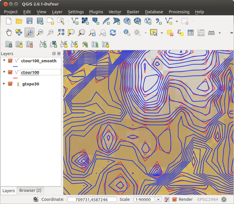
GRASS module v.generalize to smooth a vector map

Tip

Outros usos para o r.contour

The procedure described above can be used in other equivalent situations. If you have a raster map of precipitation data, for example, then the same method will be used to create a vector map of isohyetal (constant rainfall) lines.

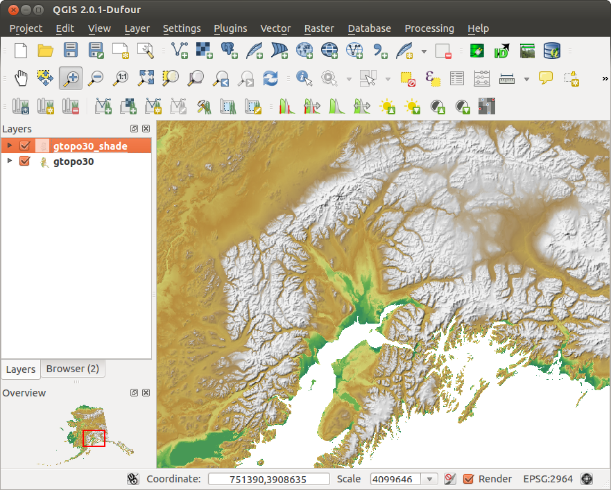
Criando um efeito de Sombras 3D¶

Several methods are used to display elevation layers and give a 3D effect to maps. The use of contour lines as shown above is one popular method often chosen to produce topographic maps. Another way to display a 3D effect is by hillshading. The hillshade effect is created from a DEM (elevation) raster by first calculating the slope and aspect of each cell, then simulating the sun’s position in the sky and giving a reflectance value to each cell. Thus you get sun facing slopes lighted and the slopes facing away from the sun (in shadow) are darkened.

• Begin this example by loading the gtopo30 elevation raster. Start the GRASS toolbox and under the Raster category double click to open Spatial analysis ‣ Terrain analysis.

• De seguida clique em r.shaded.relief para abrir o módulo.

• Change the azimuth angle 270 to 315.
• Enter gtopo30_shade for the new hillshade raster, and click [Run].
• When the process completes, add the hillshade raster to the map. You should see it displayed in grayscale.
• To view both the hill shading and the colors of the gtopo30 together shift the hillshade map below the gtopo30 map in the table of contents, then open the Properties window of gtopo30, switch to the transparency tab and set its transparency level to about 25%.

You should now have the gtopo30 elevation with its colormap and transparency setting displayed above the grayscale hillshade map. In order to see the visual effects of the hillshading, turn off the gtopo30_shade map, then turn it back on.

Usando a linha de comandos do GRASS

The GRASS plugin in QGIS is designed for users who are new to GRASS, and not familiar with all the modules and options. As such, some modules in the toolbox do not show all the options available, and some modules do not appear at all. The GRASS shell (or console) gives the user access to those additional GRASS modules that do not appear in the toolbox tree, and also to some additional options to the modules that are in the toolbox with the simplest default parameters. This example demonstrates the use of an additional option in the r.shaded.relief module that was shown above.

Figure GRASS module 5:

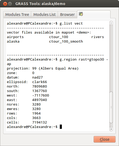
The GRASS shell, r.shaded.relief module

The module r.shaded.relief can take a parameter zmult which multiplies the elevation values relative to the X-Y coordinate units so that the hillshade effect is even more pronounced.

• Load the gtopo30 elevation raster as above, then start the GRASS toolbox and click on the GRASS shell. In the shell window type the command r.shaded.relief map=gtopo30 shade=gtopo30_shade2 azimuth=315 zmult=3 and press [Enter].
• After the process finishes shift to the Browse tab and double click on the new gtopo30_shade2 raster to display in QGIS.
• As explained above, shift the shaded relief raster below the gtopo30 raster in the Table of Contents, then check transparency of the colored gtopo30 layer. You should see that the 3D effect stands out more strongly compared to the first shaded relief map.

Figure GRASS module 6:

Displaying shaded relief created with the GRASS module r.shaded.relief

Raster statistics in a vector map¶

The next example shows how a GRASS module can aggregate raster data and add columns of statistics for each polygon in a vector map.

• Again using the Alaska data, refer to Importando dados para uma LOCALIZAÇÃO GRASS to import the trees shapefile from the shapefiles directory into GRASS.
• Now an intermediary step is required: centroids must be added to the imported trees map to make it a complete GRASS area vector (including both boundaries and centroids).
• From the toolbox choose Vector ‣ Manage features, and open the module v.centroids.
• Enter as the output vector map ‘forest_areas’ and run the module.
• Now load the forest_areas vector and display the types of forests - deciduous, evergreen, mixed - in different colors: In the layer Properties window, Symbology tab, choose from Legend type ‘Unique value’ and set the Classification field to ‘VEGDESC’. (Refer to the explanation of the symbology tab :ref:sec_symbology in the vector section).
• Next reopen the GRASS toolbox and open Vector ‣ Vector update by other maps.
• Click on the v.rast.stats module. Enter gtopo30, and forest_areas.
• Only one additional parameter is needed: Enter column prefix elev, and click [run]. This is a computationally heavy operation which will run for a long time (probably up to two hours).
• Finally open the forest_areas attribute table, and verify that several new columns have been added including elev_min, elev_max, elev_mean etc. for each forest polygon.

Working with the GRASS LOCATION browser¶

Another useful feature inside the GRASS Toolbox is the GRASS LOCATION browser. In figure_grass_module_7 you can see the current working LOCATION with its MAPSETs.

In the left browser windows you can browse through all MAPSETs inside the current LOCATION. The right browser window shows some meta information for selected raster or vector layers, e.g. resolution, bounding box, data source, connected attribute table for vector data and a command history.

Figure GRASS module 7:

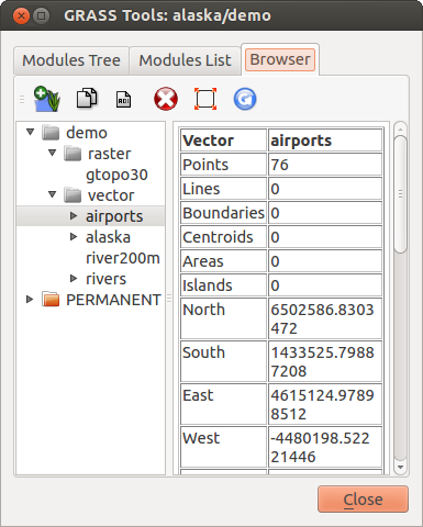
GRASS LOCATION browser

The toolbar inside the Browser tab offers following tools to manage the selected LOCATION:

• Add selected map to canvas
• Copy selected map
• Rename selected map
• Delete selected map
• Set current region to selected map
• Refresh browser window

The Rename selected map and Delete selected map only work with maps inside your currently selected MAPSET. All other tools also work with raster and vector layers in another MAPSET.

<?xml version="1.0" encoding="UTF-8"?>
<!DOCTYPE qgisgrassmodule SYSTEM "http://mrcc.com/qgisgrassmodule.dtd">

<qgisgrassmodule label="Vector buffer" module="v.buffer">
        <option key="input" typeoption="type" layeroption="layer" />
        <option key="buffer"/>
        <option key="output" />
</qgisgrassmodule>