.
Integrarea GRASS GIS
The GRASS plugin provides access to GRASS GIS databases and functionalities (see GRASS-PROJECT in Literatură și Referințe Web). This includes visualizing GRASS raster and vector layers, digitizing vector layers, editing vector attributes, creating new vector layers and analysing GRASS 2-D and 3-D data with more than 400 GRASS modules.
In this section, we’ll introduce the plugin functionalities and give some examples of managing and working with GRASS data. The following main features are provided with the toolbar menu when you start the GRASS plugin, as described in section sec_starting_grass:
 Open mapset
 New mapset
 Close mapset
 Add GRASS vector layer
 Add GRASS raster layer
 Create new GRASS vector
 Edit GRASS vector layer
 Open GRASS tools
 Display current GRASS region
 Edit current GRASS region
Startarea plugin-ului GRASS
To use GRASS functionalities and/or visualize GRASS vector and raster layers in
QGIS, you must select and load the GRASS plugin with the Plugin Manager.
Therefore, go to the menu Plugins ‣  Manage Plugins, select
  GRASS and click
[OK].
GRASS and click
[OK].
You can now start loading raster and vector layers from an existing GRASS
LOCATION (see section sec_load_grassdata). Or, you can create a new
GRASS LOCATION with QGIS (see section Crearea unei noi LOCAȚII GRASS) and import
some raster and vector data (see section Importați datele într-o LOCAȚIE GRASS) for further
analysis with the GRASS Toolbox (see section Bara de instrumente GRASS).
Încărcarea straturilor raster și vectoriale GRASS
With the GRASS plugin, you can load vector or raster layers using the appropriate
button on the toolbar menu. As an example, we will use the QGIS Alaska dataset (see
section Date eșantion). It includes a small sample GRASS LOCATION
with three vector layers and one raster elevation map.
- Create a new folder called
grassdata, download the QGIS ‘Alaska’ datasetqgis_sample_data.zipfrom http://download.osgeo.org/qgis/data/ and unzip the file intograssdata. - Start QGIS.
- If not already done in a previous QGIS session, load the GRASS plugin
clicking on Plugins ‣
Manage Plugins and activate GRASS.
The GRASS toolbar appears in the QGIS main window.
- In the GRASS toolbar, click the Open mapset icon
to bring up the MAPSET wizard.
- For
Gisdbase, browse and select or enter the path to the newly created foldergrassdata. - You should now be able to select the LOCATION

alaskaand the MAPSET demo. - Click [OK]. Notice that some previously disabled tools in the GRASS toolbar are now enabled.
- Click on Add GRASS raster layer, choose the map name
gtopo30and click [OK]. The elevation layer will be visualized. - Click on Add GRASS vector layer, choose the map name
alaskaand click [OK]. The Alaska boundary vector layer will be overlayed on top of thegtopo30map. You can now adapt the layer properties as described in chapter Dialogul Proprietăților Vectoriale (e.g., change opacity, fill and outline color). - Also load the other two vector layers,
riversandairports, and adapt their properties.
As you see, it is very simple to load GRASS raster and vector layers in QGIS.
See the following sections for editing GRASS data and creating a new LOCATION.
More sample GRASS LOCATIONs are available at the GRASS website at
http://grass.osgeo.org/download/sample-data/.
Tip
Încărcarea Datelor GRASS
If you have problems loading data or QGIS terminates abnormally, check to make sure you have loaded the GRASS plugin properly as described in section Startarea plugin-ului GRASS.
GRASS LOCATION și MAPSET
GRASS data are stored in a directory referred to as GISDBASE. This directory, often
called grassdata, must be created before you start working with the GRASS
plugin in QGIS. Within this directory, the GRASS GIS data are organized by projects
stored in subdirectories called LOCATIONs. Each LOCATION is defined
by its coordinate system, map projection and geographical boundaries. Each
LOCATION can have several MAPSETs (subdirectories of the
LOCATION) that are used to subdivide the project into different topics or
subregions, or as workspaces for individual team members (see Neteler & Mitasova
2008 in Literatură și Referințe Web). In order to analyze vector and raster layers
with GRASS modules, you must import them into a GRASS LOCATION. (This is
not strictly true – with the GRASS modules r.external and v.external
you can create read-only links to external GDAL/OGR-supported datasets without
importing them. But because this is not the usual way for beginners to work with
GRASS, this functionality will not be described here.)
Figure GRASS location 1:
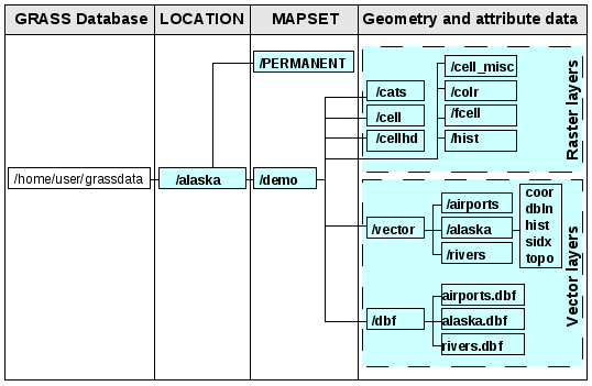
Datele GRASS din LOCAȚIA alaska
Crearea unei noi LOCAȚII GRASS
As an example, here is how the sample GRASS LOCATION alaska, which is
projected in Albers Equal Area projection with unit feet was created for the
QGIS sample dataset. This sample GRASS LOCATION alaska will be used for
all examples and exercises in the following GRASS-related sections. It is
useful to download and install the dataset on your computer (see Date eșantion).
- Start QGIS and make sure the GRASS plugin is loaded.
- Visualize the
alaska.shpshapefile (see section Loading a Shapefile) from the QGIS Alaska dataset (see Date eșantion). - In the GRASS toolbar, click on the New mapset icon
to bring up the MAPSET wizard.
Selectați dosarul
grassdata, unei baze de date existente GRASS (GISDBASE) sau creați unul pentru nouaLOCAȚIEfolosind un manager de fișiere de pe computerul dvs. Apoi faceți clic pe [Next].- We can use this wizard to create a new
MAPSETwithin an existingLOCATION(see section Adăugarea unui nou MAPSET) or to create a newLOCATIONaltogether. Select Create new
location (see figure_grass_location_2).
Create new
location (see figure_grass_location_2). Introduceți un nume pentru
LOCATION– vom folosi ‘alaska’ – apoi faceți clic pe [Next].- Define the projection by clicking on the radio button
Projection to enable the projection list.
- We are using Albers Equal Area Alaska (feet) projection. Since we happen to
know that it is represented by the EPSG ID 2964, we enter it in the search box.
(Note: If you want to repeat this process for another
LOCATIONand projection and haven’t memorized the EPSG ID, click on the CRS Status icon in the lower right-hand corner of the status bar (see
section Lucrul cu Proiecții)).
CRS Status icon in the lower right-hand corner of the status bar (see
section Lucrul cu Proiecții)). În Filtrul, inserați 2964 pentru a selecta proiecția.
Clic pe [Next].
- To define the default region, we have to enter the
LOCATIONbounds in the north, south, east, and west directions. Here, we simply click on the button [Set current |qg| extent], to apply the extent of the loaded layeralaska.shpas the GRASS default region extent. Clic pe [Next].
- We also need to define a
MAPSETwithin our newLOCATION(this is necessary when creating a newLOCATION). You can name it whatever you like - we used ‘demo’. GRASS automatically creates a specialMAPSETcalledPERMANENT, designed to store the core data for the project, its default spatial extent and coordinate system definitions (see Neteler & Mitasova 2008 in Literatură și Referințe Web). Verificați rezumatul pentru a vă asigura că este corect, apoi faceți clic pe [Finish].
Sunt create noua
LOCAȚIE, ‘alaska’, și douăSETURI DE HĂRȚI, ‘demo’ și ‘PERMANENT’. Setul deschis în mod curent este ‘demo’, așa cum a l-ați definit.Observați că unele instrumente din bara de instrumente GRASS, dezactivate anterior, sunt acum activate.
Figure GRASS location 2:
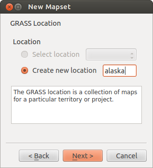
Creating a new GRASS LOCATION or a new MAPSET in QGIS
If that seemed like a lot of steps, it’s really not all that bad and a very quick
way to create a LOCATION. The LOCATION ‘alaska’ is now ready for
data import (see section Importați datele într-o LOCAȚIE GRASS). You can also use the already-existing
vector and raster data in the sample GRASS LOCATION ‘alaska’,
included in the QGIS ‘Alaska’ dataset Date eșantion, and move on to
section Modelul de date vectoriale GRASS.
Adăugarea unui nou MAPSET
A user has write access only to a GRASS MAPSET he or she created. This means that
besides access to your own MAPSET, you can read maps in other users’
MAPSETs (and they can read yours), but you can modify or remove only the maps in your own MAPSET.
All MAPSETs include a WIND file that stores the current boundary
coordinate values and the currently selected raster resolution (see Neteler & Mitasova
2008 in Literatură și Referințe Web, and section Regiunea instrumentelor GRASS).
- Start QGIS and make sure the GRASS plugin is loaded.
- In the GRASS toolbar, click on the New mapset icon
to bring up the MAPSET wizard.
Selectați folderul
grassdataal bazei de date GRASS (GISDBASE) cu locațiaLOCATION‘alaska’, în care dorim să adăugăm un nou set de hărți denumit ‘test’.Clic pe [Next].
- We can use this wizard to create a new
MAPSETwithin an existingLOCATIONor to create a newLOCATIONaltogether. Click on the radio button Select location
(see figure_grass_location_2) and click [Next]. Introduceți denumirea
textpentru noulSet de Hărți. În jos ferestrei se poate vedea listaSeturilor de Hărțiexistente, precum și proprietarii aferenți.Clic pe [Next], verificați rezumatul, pentru a vă asigura că este corect, apoi faceți clic pe [Finish].
Importați datele într-o LOCAȚIE GRASS
This section gives an example of how to import raster and vector data into the
‘alaska’ GRASS LOCATION provided by the QGIS ‘Alaska’ dataset.
Therefore, we use the landcover raster map landcover.img and the vector GML
file lakes.gml from the QGIS ‘Alaska’ dataset (see Date eșantion).
- Start QGIS and make sure the GRASS plugin is loaded.
- In the GRASS toolbar, click the Open MAPSET icon
to bring up the MAPSET wizard.
- Select as GRASS database the folder
grassdatain the QGIS Alaska dataset, asLOCATION‘alaska’, asMAPSET‘demo’ and click [OK]. - Now click the Open GRASS tools icon. The
GRASS Toolbox (see section Bara de instrumente GRASS) dialog appears.
- To import the raster map
landcover.img, click the moduler.in.gdalin the Modules Tree tab. This GRASS module allows you to import GDAL-supported raster files into a GRASSLOCATION. The module dialog forr.in.gdalappears. - Browse to the folder
rasterin the QGIS ‘Alaska’ dataset and select the filelandcover.img. - As raster output name, define
landcover_grassand click [Run]. In the Output tab, you see the currently running GRASS commandr.in.gdal -o input=/path/to/landcover.img output=landcover_grass. - When it says Succesfully finished, click [View output].
The
landcover_grassraster layer is now imported into GRASS and will be visualized in the QGIS canvas. - To import the vector GML file
lakes.gml, click the modulev.in.ogrin the Modules Tree tab. This GRASS module allows you to import OGR-supported vector files into a GRASSLOCATION. The module dialog forv.in.ograppears. - Browse to the folder
gmlin the QGIS ‘Alaska’ dataset and select the filelakes.gmlas OGR file. - As vector output name, define
lakes_grassand click [Run]. You don’t have to care about the other options in this example. In the Output tab you see the currently running GRASS commandv.in.ogr -o dsn=/path/to/lakes.gml output=lakes\_grass. - When it says Succesfully finished, click [View output]. The
lakes_grassvector layer is now imported into GRASS and will be visualized in the QGIS canvas.
Modelul de date vectoriale GRASS
It is important to understand the GRASS vector data model prior to digitizing.
In general, GRASS uses a topological vector model.
This means that areas are not represented as closed polygons, but by one or more boundaries. A boundary between two adjacent areas is digitized only once, and it is shared by both areas. Boundaries must be connected and closed without gaps. An area is identified (and labeled) by the centroid of the area.
Besides boundaries and centroids, a vector map can also contain points and lines. All these geometry elements can be mixed in one vector and will be represented in different so-called ‘layers’ inside one GRASS vector map. So in GRASS, a layer is not a vector or raster map but a level inside a vector layer. This is important to distinguish carefully. (Although it is possible to mix geometry elements, it is unusual and, even in GRASS, only used in special cases such as vector network analysis. Normally, you should prefer to store different geometry elements in different layers.)
It is possible to store several ‘layers’ in one vector dataset. For example, fields, forests and lakes can be stored in one vector. An adjacent forest and lake can share the same boundary, but they have separate attribute tables. It is also possible to attach attributes to boundaries. An example might be the case where the boundary between a lake and a forest is a road, so it can have a different attribute table.
The ‘layer’ of the feature is defined by the ‘layer’ inside GRASS. ‘Layer’ is the number which defines if there is more than one layer inside the dataset (e.g., if the geometry is forest or lake). For now, it can be only a number. In the future, GRASS will also support names as fields in the user interface.
Attributes can be stored inside the GRASS LOCATION as dBase or SQLite3 or
in external database tables, for example, PostgreSQL, MySQL, Oracle, etc.
Atributele din tabelele bazei de date sunt legate de elementele geometrice printr-o valoare de ‘categorie’.
‘Categoria’ (key, ID) este un număr întreg atașat primitivelor geometrice, fiind folosită ca legătură către o coloană cheie, din tabelul bazei de date.
Tip
Înțelegerea modelului de date vectoriale GRASS
Cel mai bun mod de a învăța despre modelul vectorial GRASS și despre capabilitățile sale, este de a descărca unul dintre multe tutoriale GRASS în care modelul vectorial este descris în profunzime. Vizitați http://grass.osgeo.org/documentation/manuals/ pentru informații suplimentare, cărți și tutoriale în diverse limbi.
Crearea unui nou strat vectorial GRASS
To create a new GRASS vector layer with the GRASS plugin, click the
Create new GRASS vector toolbar icon.
Enter a name in the text box, and you can start digitizing point, line or polygon
geometries following the procedure described in section Digitizarea și editarea unui strat vectorial GRASS.
In GRASS, it is possible to organize all sorts of geometry types (point, line and area) in one layer, because GRASS uses a topological vector model, so you don’t need to select the geometry type when creating a new GRASS vector. This is different from shapefile creation with QGIS, because shapefiles use the Simple Feature vector model (see section Crearea noillor straturi Vectoriale).
Tip
Creating an attribute table for a new GRASS vector layer
If you want to assign attributes to your digitized geometry features, make sure to create an attribute table with columns before you start digitizing (see figure_grass_digitizing_5).
Digitizarea și editarea unui strat vectorial GRASS
The digitizing tools for GRASS vector layers are accessed using the
Edit GRASS vector layer icon on the toolbar. Make sure you
have loaded a GRASS vector and it is the selected layer in the legend before
clicking on the edit tool. Figure figure_grass_digitizing_2 shows the GRASS
edit dialog that is displayed when you click on the edit tool. The tools and
settings are discussed in the following sections.
Tip
Digitizarea poligoanelor în GRASS
If you want to create a polygon in GRASS, you first digitize the boundary of the polygon, setting the mode to ‘No category’. Then you add a centroid (label point) into the closed boundary, setting the mode to ‘Next not used’. The reason for this is that a topological vector model links the attribute information of a polygon always to the centroid and not to the boundary.
Bara de Instrumente
In figure_grass_digitizing_1, you see the GRASS digitizing toolbar icons provided by the GRASS plugin. Table table_grass_digitizing_1 explains the available functionalities.
Figure GRASS digitizing 1:

GRASS Digitizing Toolbar
Pictogramă |
Instrument |
Scop |
|---|---|---|
 |
Punct Nou |
Digitizare punct nou |
 |
Linie nouă |
Digitizare linie nouă |
 |
Limită Nouă |
Digitize new boundary (finish by selecting new tool) |
 |
Centroid Nou |
Digitizarea unui nou centroid (etichetarea zonei existente) |
 |
Move vertex | Move one vertex of existing line or boundary and identify new position |
 |
Add vertex | Add a new vertex to existing line |
 |
Delete vertex | Delete vertex from existing line (confirm selected vertex by another click) |
 |
Move element | Move selected boundary, line, point or centroid and click on new position |
 |
Split line | Split an existing line into two parts |
 |
Delete element | Delete existing boundary, line, point or centroid (confirm selected element by another click) |
 |
Edit attributes | Edit attributes of selected element (note that one element can represent more features, see above) |
 |
Close | Close session and save current status (rebuilds topology afterwards) |
Tabela 1 de Digitizare GRASS: Insrtrumente de Digitizare GRASS
Category Tab
The Category tab allows you to define the way in which the category values will be assigned to a new geometry element.
Figure GRASS digitizing 2:
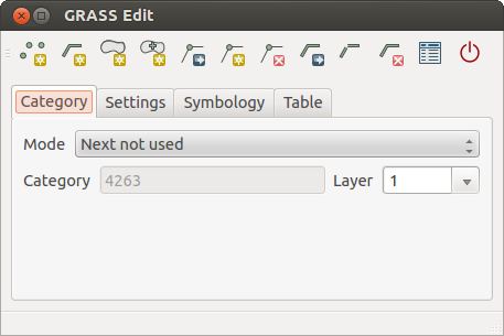
GRASS Digitizing Category Tab
- Mode: The category value that will be applied to new geometry elements.
- Next not used - Apply next not yet used category value to geometry element.
- Manual entry - Manually define the category value for the geometry element in the ‘Category’ entry field.
- No category - Do not apply a category value to the geometry element. This is used, for instance, for area boundaries, because the category values are connected via the centroid.
- Category - The number (ID) that is attached to each digitized geometry element. It is used to connect each geometry element with its attributes.
- Field (layer) - Each geometry element can be connected with several attribute tables using different GRASS geometry layers. The default layer number is 1.
Tip
Creating an additional GRASS ‘layer’ with |qg|
If you would like to add more layers to your dataset, just add a new number in the ‘Field (layer)’ entry box and press return. In the Table tab, you can create your new table connected to your new layer.
Settings Tab
The Settings tab allows you to set the snapping in screen pixels. The threshold defines at what distance new points or line ends are snapped to existing nodes. This helps to prevent gaps or dangles between boundaries. The default is set to 10 pixels.
Figure GRASS digitizing 3:
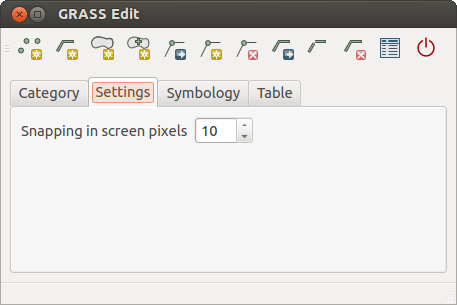
GRASS Digitizing Settings Tab
Symbology Tab
The Symbology tab allows you to view and set symbology and color settings for various geometry types and their topological status (e.g., closed / opened boundary).
Figure GRASS digitizing 4:
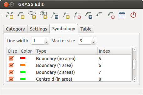
GRASS Digitizing Symbology Tab
Table Tab
The Table tab provides information about the database table for a given ‘layer’. Here, you can add new columns to an existing attribute table, or create a new database table for a new GRASS vector layer (see section Crearea unui nou strat vectorial GRASS).
Figure GRASS digitizing 5:
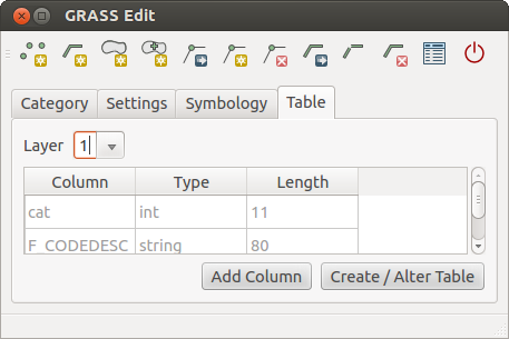
GRASS Digitizing Table Tab
Tip
Permisiuni de Editare GRASS
Trebuie să fiți proprietarul SETULUI DE HĂRȚI GRASS, pentru a-l putea edita. Este imposibilă editarea datelor din straturile SETULUI DE HĂRȚI care nu vă aparține, chiar dacă aveți permisiunea de scriere.
Regiunea instrumentelor GRASS
The region definition (setting a spatial working window) in GRASS is important
for working with raster layers. Vector analysis is by default not limited to any
defined region definitions. But all newly created rasters will have the spatial
extension and resolution of the currently defined GRASS region, regardless of
their original extension and resolution. The current GRASS region is stored in
the $LOCATION/$MAPSET/WIND file, and it defines north, south, east and
west bounds, number of columns and rows, horizontal and vertical spatial resolution.
It is possible to switch on and off the visualization of the GRASS region in the QGIS
canvas using the Display current GRASS region button.
With the Edit current GRASS region icon, you can open
a dialog to change the current region and the symbology of the GRASS region
rectangle in the QGIS canvas. Type in the new region bounds and resolution, and
click [OK]. The dialog also allows you to select a new region interactively with your
mouse on the QGIS canvas. Therefore, click with the left mouse button in the QGIS
canvas, open a rectangle, close it using the left mouse button again and click
[OK].
The GRASS module g.region provides a lot more parameters to define an
appropriate region extent and resolution for your raster analysis. You can use
these parameters with the GRASS Toolbox, described in section Bara de instrumente GRASS.
Bara de instrumente GRASS
The Open GRASS Tools box provides GRASS module functionalities
to work with data inside a selected GRASS LOCATION and MAPSET.
To use the GRASS Toolbox you need to open a LOCATION and MAPSET
that you have write permission for (usually granted, if you created the MAPSET).
This is necessary, because new raster or vector layers created during analysis
need to be written to the currently selected LOCATION and MAPSET.
Figure GRASS Toolbox 1:
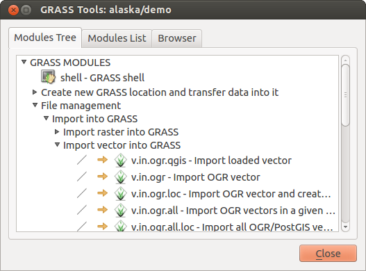
Bara de Instrumente și Arborele Modulelor GRASS 
Lucrul cu modulele GRASS
The GRASS shell inside the GRASS Toolbox provides access to almost all (more than 300) GRASS modules in a command line interface. To offer a more user-friendly working environment, about 200 of the available GRASS modules and functionalities are also provided by graphical dialogs within the GRASS plugin Toolbox.
A complete list of GRASS modules available in the graphical Toolbox in QGIS version 2.8 is available in the GRASS wiki at http://grass.osgeo.org/wiki/GRASS-QGIS_relevant_module_list.
De asemenea, este posibilă personalizarea conținutul Instrumentarului GRASS. Această procedură este descrisă în secțiunea Personalizarea Barei de Instrumente GRASS.
As shown in figure_grass_toolbox_1, you can look for the appropriate GRASS module using the thematically grouped Modules Tree or the searchable Modules List tab.
By clicking on a graphical module icon, a new tab will be added to the Toolbox dialog, providing three new sub-tabs: Options, Output and Manual.
Opțiuni
The Options tab provides a simplified module dialog where you can usually select a raster or vector layer visualized in the QGIS canvas and enter further module-specific parameters to run the module.
Figure GRASS module 1:
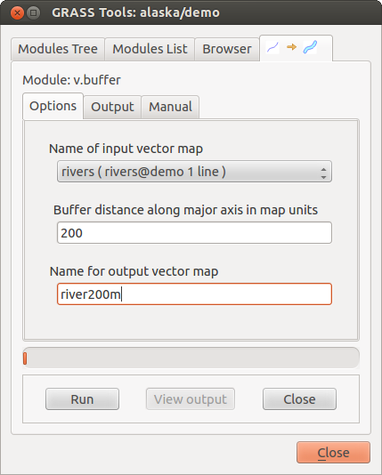
Opțiunile Bării de Instrumente și a Arborelui Modulelor GRASS
The provided module parameters are often not complete to keep the dialog clear. If you want to use further module parameters and flags, you need to start the GRASS shell and run the module in the command line.
A new feature since QGIS 1.8 is the support for a Show Advanced Options
button below the simplified module dialog in the Options tab. At the
moment, it is only added to the module v.in.ascii as an example of use, but it will
probably be part of more or all modules in the GRASS Toolbox in future versions
of QGIS. This allows you to use the complete GRASS module options without the need
to switch to the GRASS shell.
Rezultat
Figure GRASS module 2:
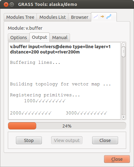
Rezultatul Bării de Instrumente și a Arborelui Modulelor GRASS
Fila Rezultatelor oferă informații despre starea de ieșire a modulului. Când faceți clic pe butonul [Run], modulul comută la fila Rezultatelor tab, apoi veți vedea informații despre procesul de analiză. Dacă totul funcționează bine, veți vedea în cele din urmă un mesaj de Definitivare cu succes.
Manual
Figure GRASS module 3:
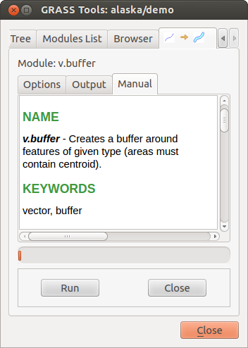
Manualul Bării de Instrumente și a Arborelui Modulelor GRASS
The Manual tab shows the HTML help page of the GRASS module. You can
use it to check further module parameters and flags or to get a deeper knowledge
about the purpose of the module. At the end of each module manual page, you see
further links to the Main Help index, the Thematic index and the
Full index. These links provide the same information as the
module g.manual.
Tip
Afișează imediat rezultatele
Dacă doriți să afișați imediat rezultatele calculelor dvs în canevasul hărții, puteți folosi butonul ‘Vizualizare Output’, din partea de jos a filei modulului.
Exemple de module GRASS
Următoarele exemple vor demonstra puterea unora dintre modulele GRASS.
Crearea curbelor de nivel
The first example creates a vector contour map from an elevation raster (DEM).
Here, it is assumed that you have the Alaska LOCATION set up as explained in section
Importați datele într-o LOCAȚIE GRASS.
- First, open the location by clicking the
Open mapset button and choosing the Alaska location.
- Now load the
gtopo30elevation raster by clicking Add GRASS raster layer and selecting the
gtopo30raster from the demo location. - Now open the Toolbox with the Open GRASS tools button.
În lista de de unelte pentru categorii, faceți dublu-clic pe Raster ‣ Surface Management ‣ Generate vector contour lines.
- Now a single click on the tool r.contour will open the tool dialog as
explained above (see Lucrul cu modulele GRASS). The
gtopo30raster should appear as the Name of input raster. - Type into the Increment between Contour levels
 the value 100. (This will create contour lines at intervals of 100 meters.)
 Introduceți în Name for output vector map `numele ``ctour_100`.
Faceți clic pe [Run] pentru a începe procesul. Așteptați câteva momente până când mesajul
Finalizare cu succesapare în fereastra de ieșire. Apoi faceți clic pe [View Output] și [Close].
Deoarece aceasta este o regiune de mare, va dura ceva timp până la afișare. Dupa ce se termină randarea, puteți deschide fereastra de proprietăți ale stratului pentru a schimba culoarea liniei, astfel încât conturul să apară clar pe rasterul de elvație, la fel ca în Dialogul Proprietăților Vectoriale.
Next, zoom in to a small, mountainous area in the center of Alaska. Zooming in close, you will notice that the contours have sharp corners. GRASS offers the v.generalize tool to slightly alter vector maps while keeping their overall shape. The tool uses several different algorithms with different purposes. Some of the algorithms (i.e., Douglas Peuker and Vertex Reduction) simplify the line by removing some of the vertices. The resulting vector will load faster. This process is useful when you have a highly detailed vector, but you are creating a very small-scale map, so the detail is unnecessary.
Tip
Instrumentul de simplificare
Note that the QGIS fTools plugin has a Simplify geometries ‣ tool that works just like the GRASS v.generalize Douglas-Peuker algorithm.
However, the purpose of this example is different. The contour lines created by
r.contour have sharp angles that should be smoothed. Among the v.generalize
algorithms, there is Chaiken’s, which does just that (also Hermite splines). Be
aware that these algorithms can add additional vertices to the vector,
causing it to load even more slowly.
- Open the GRASS Toolbox and double-click the categories Vector ‣ Develop map ‣ Generalization, then click on the v.generalize module to open its options window.
Verificați dacă ‘ctour_100’ apare ca Nume pentru vectorul de intrare.
- From the list of algorithms, choose Chaiken’s. Leave all other options at their default, and scroll down to the last row to enter in the field Name for output vector map ‘ctour_100_smooth’, and click [Run].
- The process takes several moments. Once
Successfully finishedappears in the output windows, click [View output] and then [Close]. Puteți schimba culoarea vectorului pentru a-l afișa în mod clar pe fundalul raster, și pentru a contrasta față de curbele de nivel originale. Veți observa că noile curbe de nivel au colțuri mai fine decât originalul, în timp ce urmează fidel forma originală.
Figure GRASS module 4:
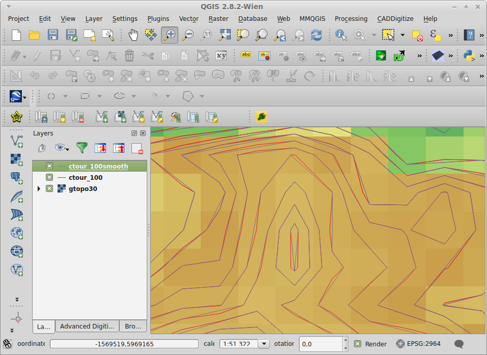
Modulul GRASS v.generalize pentru a radina o hartă vectorială
Tip
Alte utilizări pentru r.contour
The procedure described above can be used in other equivalent situations. If you have a raster map of precipitation data, for example, then the same method will be used to create a vector map of isohyetal (constant rainfall) lines.
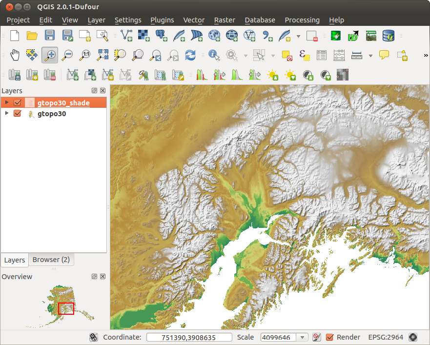
Crearea unui efect 3-D de umbrire
Several methods are used to display elevation layers and give a 3-D effect to maps. The use of contour lines, as shown above, is one popular method often chosen to produce topographic maps. Another way to display a 3-D effect is by hillshading. The hillshade effect is created from a DEM (elevation) raster by first calculating the slope and aspect of each cell, then simulating the sun’s position in the sky and giving a reflectance value to each cell. Thus, you get sun-facing slopes lighted; the slopes facing away from the sun (in shadow) are darkened.
- Begin this example by loading the
gtopo30elevation raster. Start the GRASS Toolbox, and under the Raster category, double-click to open Spatial analysis ‣ Terrain analysis. Apoi faceți clic pe r.shaded.relief pentru a deschide modulul.
- Change the azimuth angle 270 to 315.
Introduceți
gtopo30_shadepentru noul raster reliefat, apoi faceți clic pe [Run].Când procesul se încheie, adăugați hărții rasterul reliefat. Ar trebui să-l vedeți afișat în tonuri de gri.
- To view both the hillshading and the colors of the
gtopo30together, move the hillshade map below thegtopo30map in the table of contents, then open the Properties window ofgtopo30, switch to the Transparency tab and set its transparency level to about 25%.
Ar trebui să aveți acum elevația gtopo30 cu harta de cuori și transparența setate deasupra hărții reliefului, în tonuri de gri. Pentru a observa mai bine efectele vizuale ale reliefării, desetați vizualizarea hărții gtopo30_shade, apoi resetați-o.
Folosirea consolei GRASS
The GRASS plugin in QGIS is designed for users who are new to GRASS and not familiar with all the modules and options. As such, some modules in the Toolbox do not show all the options available, and some modules do not appear at all. The GRASS shell (or console) gives the user access to those additional GRASS modules that do not appear in the Toolbox tree, and also to some additional options to the modules that are in the Toolbox with the simplest default parameters. This example demonstrates the use of an additional option in the r.shaded.relief module that was shown above.
Figure GRASS module 5:
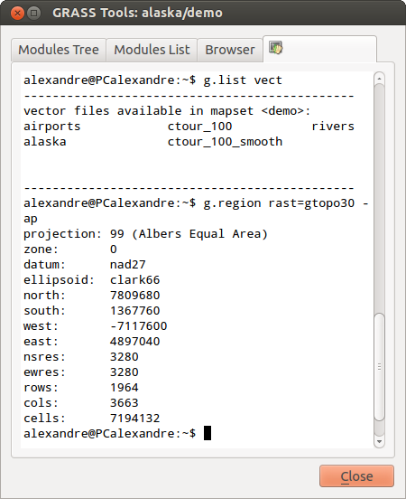
Consola GRASS, modulul r.shaded.relief
The module r.shaded.relief can take a parameter zmult, which multiplies
the elevation values relative to the X-Y coordinate units so that the hillshade
effect is even more pronounced.
- Load the
gtopo30elevation raster as above, then start the GRASS Toolbox and click on the GRASS shell. In the shell window, type the commandr.shaded.relief map=gtopo30 shade=gtopo30_shade2 azimuth=315 zmult=3and press [Enter]. - After the process finishes, shift to the Browse tab and double-click
on the new
gtopo30_shade2raster to display it in QGIS. - As explained above, move the shaded relief raster below the
gtopo30raster in the table of contents, then check the transparency of the coloredgtopo30layer. You should see that the 3-D effect stands out more strongly compared with the first shaded relief map.
Figure GRASS module 6:
Afișează relieful umbrit, creat cu modulul GRASS r.shaded.relief
Statistici raster pentru o hartă vectorială
Următorul exemplu arată modul în care un modul din GRASS poate agrega datele rastere, apoi să adauge coloanele de statistici pentru fiecare poligon din harta vectorială.
Din nou, folosind datele pentru Alaska, referiți-vă la Importați datele într-o LOCAȚIE GRASS pentru a importa arborii fișierelor shape din directorul
shapefilesdin GRASS.- Now an intermediate step is required: centroids must be added to the imported trees map to make it a complete GRASS area vector (including both boundaries and centroids).
Din Bara de instrumente alegeți Vector ‣ Manage features, apoi deschideți modulul v.centroids.
Introduceți ‘forest_areas’ pentru output vector map, apoi rulați modulul.
- Now load the
forest_areasvector and display the types of forests - deciduous, evergreen, mixed - in different colors: In the layer Properties window, Symbology tab, choose from Legend type ‘Unique value’ and set the Classification field
to ‘VEGDESC’. (Refer to the explanation of the symbology tab in
Meniul Stilului of the vector section.) Mai departe, redeschideți Bara de instrumente GRASS, apoi deschideți Vector ‣ Vector update din alte hărți.
Clic pe modulul v.rast.stats. Introduceți
gtopo30șiforest_areas.- Only one additional parameter is needed: Enter column prefix
elev, and click [Run]. This is a computationally heavy operation, which will run for a long time (probably up to two hours). - Finally, open the
forest_areasattribute table, and verify that several new columns have been added, includingelev_min,elev_max,elev_mean, etc., for each forest polygon.
Working with the GRASS LOCATION browser
Another useful feature inside the GRASS Toolbox is the GRASS LOCATION
browser. In figure_grass_module_7, you can see the current working LOCATION
with its MAPSETs.
In the left browser windows, you can browse through all MAPSETs inside the
current LOCATION. The right browser window shows some meta-information
for selected raster or vector layers (e.g., resolution, bounding box, data source,
connected attribute table for vector data, and a command history).
Figure GRASS module 7:
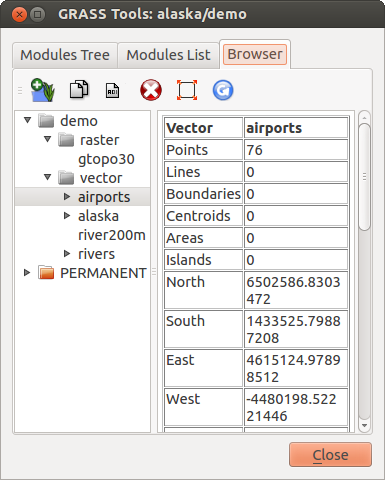
GRASS LOCATION browser
The toolbar inside the Browser tab offers the following tools to manage
the selected LOCATION:
 Add selected map to canvas
 Copy selected map
 Rename selected map
 Delete selected map
 Set current region to selected map
 Refresh browser window
The Rename selected map and
Delete selected map only work with maps inside your currently selected
MAPSET. All other tools also work with raster and vector layers in
another MAPSET.
Personalizarea Barei de Instrumente GRASS
Nearly all GRASS modules can be added to the GRASS Toolbox. An XML interface is provided to parse the pretty simple XML files that configure the modules’ appearance and parameters inside the Toolbox.
Un fișier XML eșantion, pentru generarea modulului v.buffer (v.buffer.qgm) arată în felul următor:
<?xml version="1.0" encoding="UTF-8"?>
<!DOCTYPE qgisgrassmodule SYSTEM "http://mrcc.com/qgisgrassmodule.dtd">

<qgisgrassmodule label="Vector buffer" module="v.buffer">
        <option key="input" typeoption="type" layeroption="layer" />
        <option key="buffer"/>
        <option key="output" />
</qgisgrassmodule>
The parser reads this definition and creates a new tab inside the Toolbox when you select the module. A more detailed description for adding new modules, changing a module’s group, etc., can be found on the QGIS wiki at http://hub.qgis.org/projects/quantum-gis/wiki/Adding_New_Tools_to_the_GRASS_Toolbox.