The graphical modeler¶

Definition of inputs¶

The first step to create a model is to define the inputs it needs. The following elements are found in the Inputs tab on the left side of the modeler window:

• Raster layer
• Vector layer
• String
• Table field
• Table
• Extent
• Number
• Boolean
• File

Double-clicking on any of them, a dialog is shown to define its characteristics. Depending on the parameter itself, the dialog will contain just one basic element (the description, which is what the user will see when executing the model) or more of them. For instance, when adding a numerical value, as it can be seen in the next figure, apart from the description of the parameter you have to set a default value and a range of valid values.

Figure Processing 17:

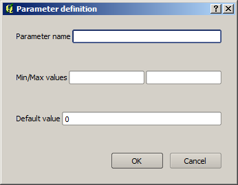
Model Parameters

For each added input, a new element is added to the modeler canvas.

Figure Processing 18:

Model Parameters

Definition of the workflow¶

Once the inputs have been defined, it is time to define the algorithms to apply on them. Algorithms can be found in the Algorithms tab, grouped much in the same way as they are in the toolbox.

Figure Processing 19:

Model Parameters

The appearance of the toolbox has two modes here as well: simplified and advanced. However, there is no element to switch between views in the modeler, and you have to do it in the toolbox. The mode that is selected in the toolbox is the one that will be used for the list of algorithms in the modeler.

To add an algorithm to a model, double-click on its name. An execution dialog will appear, with a content similar to the one found in the execution panel that is shown when executing the algorithm from the toolbox. The one shown next correspond to the SAGA ‘Convergence index’ algorithm, the same one we saw in the section dedicated to the toolbox.

Figure Processing 20:

Model Parameters

As you can see, some differences exist. Instead of the file output box that was used to set the filepath for output layers and tables, a simple text box is. If the layer generated by the algorithm is just a temporary result that will be used as the input of another algorithm and should not be kept as a final result, just do not edit that text box. Typing anything on it means that the result is a final one, and the text that you supply will be the description for the output, which will be the one the user will see when executing the model.

Selecting the value of each parameter is also a bit different, since there are important differences between the context of the modeler and the toolbox one. Let’s see how to introduce the values for each type of parameter.

• Layers (raster and vector) and tables. They are selected from a list, but in this case the possible values are not the layers or tables currently loaded in QGIS, but the list of model inputs of the corresponding type, or other layers or tables generated by algorithms already added to the model.
• Numerical values. Literal values can be introduced directly on the text box. But this text box is also a list that can be used to select any of the numerical value inputs of the model. In this case, the parameter will take the value introduced by the user when executing the model.
• String. Like in the case of numerical values, literal strings can be typed, or an input string can be selected.
• Table field. The fields of the parent table or layer cannot be known at design-time, since they depend of the selection of the user each time the model is executed. To set the value for this parameter, type the name of a field directly in the text box, or use the list to select a table field input already added to the model. The validity of the selected field will be checked at run-time.

In all cases, you will find an additional parameter named Parent algorithms that is not available when calling the algorithm from the toolbox. This parameter allows you to define the order in which algorithms are executed, by explicitly defining one algorithm as a parent of the current one, which will force it to be executed before it.

When you use the output of a previous algorithm as the input of your algorithm, that implicitly sets the former as parent of the current one (and places the corresponding arrow in the modeler canvas). However, in some cases an algorithm might depend on another one even if it does not use any output object from it (for instance, and algorithm that executes an SQL sentence on a PostGIS database and another one which imports a layer into that same database) In that case, just select it in the Parent algorithms parameter and they will be executed in the correct order.

Once all the parameter have been assigned valid values, click on [OK] and the algorithm will be added to the canvas. It will be linked to all the other elements in the canvas, whether algorithms or inputs, which provide objects that are used as inputs for that algorithm.

Figure Processing 21:

Model Parameters

Elements can be dragged to a different position within the canvas, to change the way the module structure is displayed and make it more clear and intuitive. Links between elements are update automatically.

You can run your algorithm anytime clicking on the [Run] button. However, in order to use it from the toolbox, it has to be saved and the modeler dialog closed, to allow the toolbox to refresh its contents.

Saving and loading models¶

Use the [Save] button to save the current model and the [Open] one to open any model previously saved. Model are saved with the .model extension. If the model has been previously saved from the modeler window, you will not be prompted for a filename, since there is already a file associated with that model, and it will be used.

Before saving a model, you have to enter a name and a group for it, using the text boxes in the upper part of the window.

Models saved on the models folder (the default folder when you are prompted for a filename to save the model) will appear in the toolbox in the corresponding branch. When the toolbox is invoked, it searches the models folder for files with .model extension and loads the models they contain. Since a model is itself an algorithm, it can be added to the toolbox just like any other algorithm.

The models folder can be set from the processing configuration dialog, under the Modeler group.

Models loaded from the models folder appear not only in the toolbox, but also in the algorithms tree in the Algorithms tab of the modeler window. That means that you can incorporate a model as a part of a bigger model, just as you add any other algorithm.

In some cases, a model might not be loaded because not all the algorithms included in its workflow are available. If you have used a given algorithm as part of your model, it should be available (that is, it should appear on the toolbox) in order to load that model. Deactivating an algorithm provider in the processing configuration window renders all the algorithms in that provider unusable by the modeler, which might cause problems when loading models. Keep that in mind when you have trouble loading or executing models.

Editing a model¶

You can edit the model you are currently creating, redefining the workflow and the relationships between the algorithms and inputs that define the model itself.

If you right-click on an algorithm in the canvas representing the model, you will see a context menu like the one shown next:

Figure Processing 22:

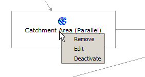
Modeler Right Click

Selecting the Remove option will cause the selected algorithm to be removed. An algorithm can be removed only if there are no other algorithms depending on it. That is, if no output from the algorithm is used in a different one as input. If you try to remove an algorithm that has others depending on it, a warning message like the one you can see below will be shown:

Figure Processing 23:

Cannot Delete Algorithm

Selecting the Edit option or simply double-clicking on the algorithm icon will show the parameters dialog of the algorithm, so you can change the inputs and parameter values. Not all input elements available in the model will appear in this case as available inputs. Layers or values generated at a more advanced step in the workflow defined by the model will not be available if they cause circular dependencies.

Select the new values and then click on the [OK] button as usual. The connections between the model elements will change accordingly in the modeler canvas.

Activating and deactivating algorithms¶

Algorithms can be deactivated in the modeler, so they will not be executed once the model is run. This can be used to test just a given part of the model, or when you do not need all the outputs it generates.

To deactivate an algorithm, right-click on its icon in the model canvas and select the Deactivate option. You will see that the algorithm is represented now with a red label under its name indicating that is not active.

Figure Processing 24:

Deactivate

All algorithms depending (directly or undirectly) on that algorithm will also appear as inactive, since they cannot be executed now.

To activate an algorithm, just right–click on its icon and select the Activate option.

Editing model help files and meta-information¶

You can document your models from the modeler itself. Just click on the [Edit model help] button and a dialog like the one shown next will appear.

Figure Processing 25:

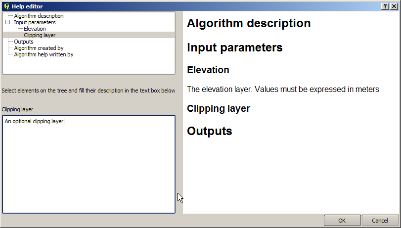
Help Edition

On the right-hand side you will see a simple HTML page, created using the description of the input parameters and outputs of the algorithm, along with some additional items like a general description of the model or its author. The first time you open the help editor all those descriptions are empty, but you can edit them using the elements on the left-hand side of the dialog. Select an element on the upper part and the write its description in the text box below.

Model help is saved in a file in the same folder as the model itself. You do not have to worry about saving it, since it is done automatically.

About available algorithms¶

You might notice that some algorithms that can be be executed from the toolbox do not appear in the list of available ones when you are designing a model. To be included in a model, and algorithm must have a correct semantic, so as to be properly linked to other in the workflow. If an algorithm does not have such well-defined semantic (for instance, if the number of output layers cannot be know in advance), then it is not possible to use it within a model, and thus does not appear in the list of them that you can find in the modeler dialog.

Additionally, you will see some algorithms in the modeler that are not found in the toolbox. This algorithms are meant to be used exclusively as part of a model, and they are of no interest in a different context. The ‘Calculator’ algorithm is an example of that. It is just a simple arithmetic calculator that you can use to modify numerical values (entered by the user or generated by some other algorithm). This tools is really useful within a model, but outside of that context, it doesn’t make too much sense.

Saving models as Python code¶

Given a model, it is possible to automatically create Python code that performs the same task as the model itself. This code is used to create a console script (we will explain them later in this manual) and you can modify that script to incorporate actions and methods not available in the graphical modeler, such as loops or conditional sentences.

This feature is also a very practical way of learning how to use processign algorithms from the console and how to create new algorithms using Python code, so you can use it as a learning tool when you start creating your own scripts.

Save your model in the models folder and go to the toolbox, where it should appear now, ready to be run. Right click on the model name and select Save as Python script in the context menu that will pop-up. A dialog will prompt you to introduce the file where you want to save the script.