17. Working with Mesh Data

17.1. What’s a mesh?

A mesh is an unstructured grid usually with temporal and other components. The spatial component contains a collection of vertices, edges and/or faces, in 2D or 3D space:

• vertices - XY(Z) points (in the layer’s coordinate reference system)

• edges - connect pairs of vertices

• faces - a face is a set of edges forming a closed shape - typically a triangle or a quadrilateral (quad), rarely polygons with more vertices

Relying on the above, mesh layers can thus have different types of structure:

• 1D Meshes: consist of vertices and edges. An edge connects two vertices and can have assigned data (scalars or vectors) on it. The 1D mesh network can be for example used for modelling of an urban drainage system.

• 2D meshes: consist of faces with triangles, regular or unstructured quads.

• 3D layered meshes: consist of multiple stacked 2D unstructured meshes each extruded in the vertical direction (levels) by means of a vertical coordinate. The vertices and faces have the same topology in each vertical level. The mesh definition (vertical level extrusion) could in general change in time. The data is usually defined in volume centres or by some parametric function.

Fig. 17.1 Different mesh types

Mesh provides information about the spatial structure. In addition, the mesh can have datasets (groups) that assign a value to every vertex. For example, having a triangular mesh with numbered vertices as shown in the image below:

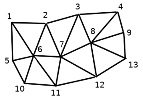
Fig. 17.2 Triangular grid with numbered vertices

Each vertex can store different datasets (typically multiple quantities), and those datasets can also have a temporal dimension. Thus, a single file may contain multiple datasets.

The following table gives an idea about the information that can be stored in mesh datasets. Table columns represent indices of mesh vertices, each row represents one dataset. Datasets can have different datatypes. In this case, it stores wind velocity at 10m at a particular moments in time (t1, t2, t3).

In a similar way, the mesh dataset can also store vector values for each vertex. For example, wind direction vector at the given time stamps:

10 metre wind	1	2	3	…
10 metre speed at time=t1	17251	24918	32858	…
10 metre speed at time=t2	19168	23001	36418	…
10 metre speed at time=t3	21085	30668	17251	…
…	…	…	…	…
10m wind direction time=t1	[20,2]	[20,3]	[20,4.5]	…
10m wind direction time=t2	[21,3]	[21,4]	[21,5.5]	…
10m wind direction time=t3	[22,4]	[22,5]	[22,6.5]	…
…	…	…	…	…

We can visualize the data by assigning colors to values (similarly to how it is done with Singleband pseudocolor raster rendering) and interpolating data between vertices according to the mesh topology. It is common that some quantities are 2D vectors rather than being simple scalar values (e.g. wind direction). For such quantities it is desirable to display arrows indicating the directions.

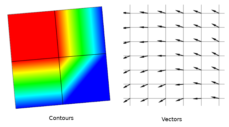
Fig. 17.3 Possible visualisation of mesh data

17.2. Supported formats

QGIS accesses mesh data using the MDAL drivers, and natively supports a variety of formats. Whether QGIS can edit a mesh layer depends on the format and the mesh structure type.

To load a mesh dataset into QGIS, use the Mesh tab in the Data Source Manager dialog. Read Loading a mesh layer for more details.

17.3. Mesh Dataset Properties

The Layer Properties dialog for a mesh layer provides general settings to manage dataset groups of the layer and their rendering (active dataset groups, symbology, 2D and 3D rendering). It also provides information about the layer.

To access the Layer Properties dialog:

• In the Layers panel, double-click the layer or right-click and select Properties… from the pop-up menu;

• Go to Layer ► Layer Properties… menu when the layer is selected.

The mesh Layer Properties dialog provides the following sections:

Information	Source	Symbology[1]
3D View[1]	Temporal	Rendering
Metadata

^[1] Also available in the Layer styling panel

Note

Most of the properties of a mesh layer can be saved to or loaded from a .qml using the Style menu at the bottom of the dialog. More details at Managing Custom Styles.

17.3.1. Information Properties

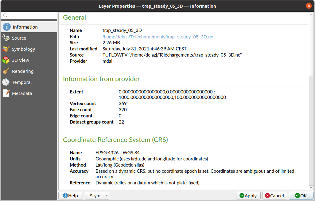
Fig. 17.4 Mesh Layer Information Properties

The Information tab is read-only and represents an interesting place to quickly grab summarized information and metadata on the current layer. Provided information are:

• general such as name in the project, source path, list of auxiliary files, last save time and size, the used provider

• based on the provider of the layer: extent, vertex, face, edges and/or dataset groups count

• the Coordinate Reference System: name, units, method, accuracy, reference (i.e. whether it’s static or dynamic)

• extracted from filled metadata: access, extents, links, contacts, history…

17.3.2. Source Properties

The Source tab displays basic information about the selected mesh, including:

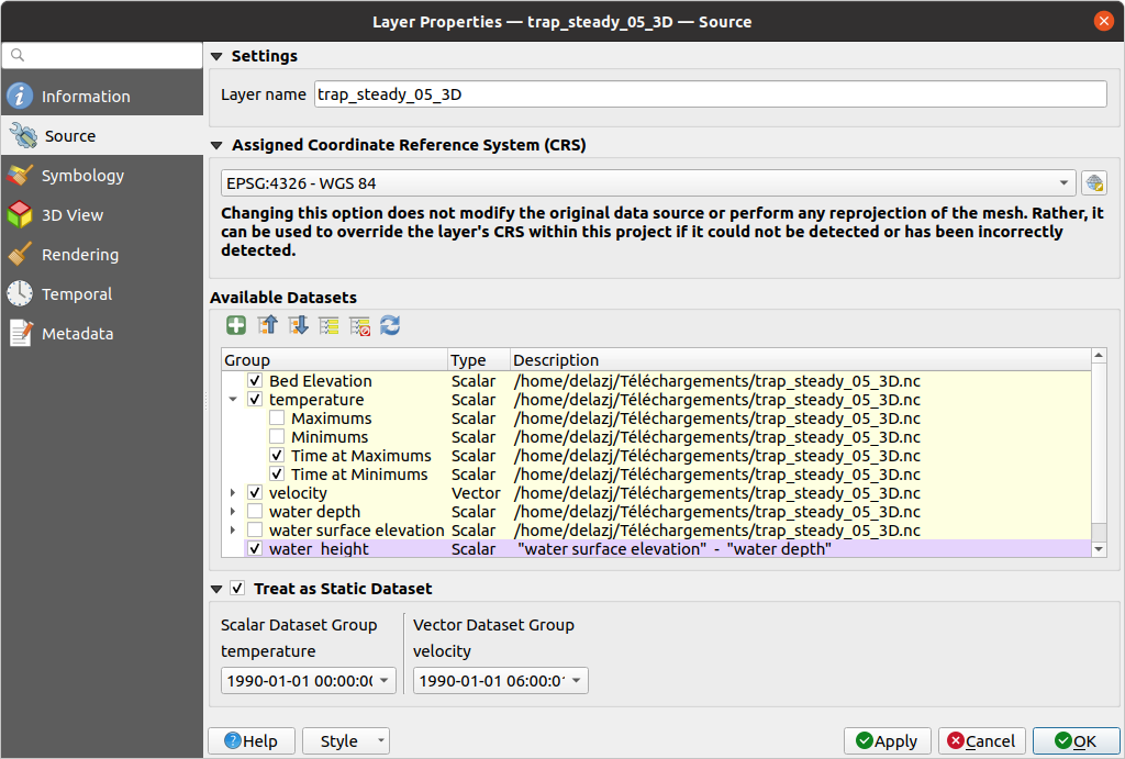
Fig. 17.5 Mesh Layer Source Properties

• the layer name to display in the Layers panel

• setting the Coordinate Reference System: Displays the layer’s Assigned Coordinate Reference System (CRS). You can change the layer’s CRS by selecting a recently used one in the drop-down list or clicking on Select CRS button (see Coordinate Reference System Selector). Use this process only if the CRS applied to the layer is wrong or if none was applied.

• The Available datasets frame lists all the dataset groups (and subgroups) in the mesh layer, with their type and description in a tree view. Both regular datasets (i.e. their data is stored in the file) and virtual datasets (which are calculated on the fly) are listed.

  • Use the Assign extra dataset to mesh button to add more groups to the current mesh layer.

  • Collapse all and Expand all the dataset tree, in case of embedded groups

  • If you are interested in few datasets, you can uncheck the others and make them unavailable in the project

  • Double-click over a name and you can rename the dataset.

  • Reset to defaults: checks all the groups and renames them back to their original name in the provider.

  • Right-click over a virtual dataset group and you can:

    • Remove dataset group from the project

    • Save dataset group as… a file on disk, to any supported format. The new file is kept assigned to the current mesh layer in the project.

• Checking the Treat as static dataset group allows to ignore the map temporal navigation properties while rendering the mesh layer. For each active dataset group (as selected in Symbology ► Datasets tab), you can:

  • set to None: the dataset group is not displayed at all

  • Display dataset: eg, for the “bed elevation” dataset which is not time aware

  • extract a particular date time: the dataset matching the provided time is rendered and stay fixed during map navigation.

17.3.3. Symbology Properties

Click the Symbology button to activate the dialog. Symbology properties are divided into several tabs:

• Datasets

• Contours

• Vectors

• Rendering

• Stacked mesh averaging method

17.3.3.1. Datasets

The tab ^Datasets is the main place to control and set which datasets will be used for the layer. It presents the following items:

• Groups available in the mesh dataset, with whether they provide:

  • scalar dataset

  • or vector dataset: by default, each vector dataset has a scalar dataset representing its magnitude automatically generated.

  Click on the icon next to the dataset name to select the group and type of data to represent.

• Selected dataset group(s) metadata, with details on:

  • the mesh type: edges or faces

  • the data type: vertices, edges, faces or volume

  • whether it’s of vector type or not

  • the original name in the mesh layer

  • the unit, if applicable

• blending mode available for the selected datasets.

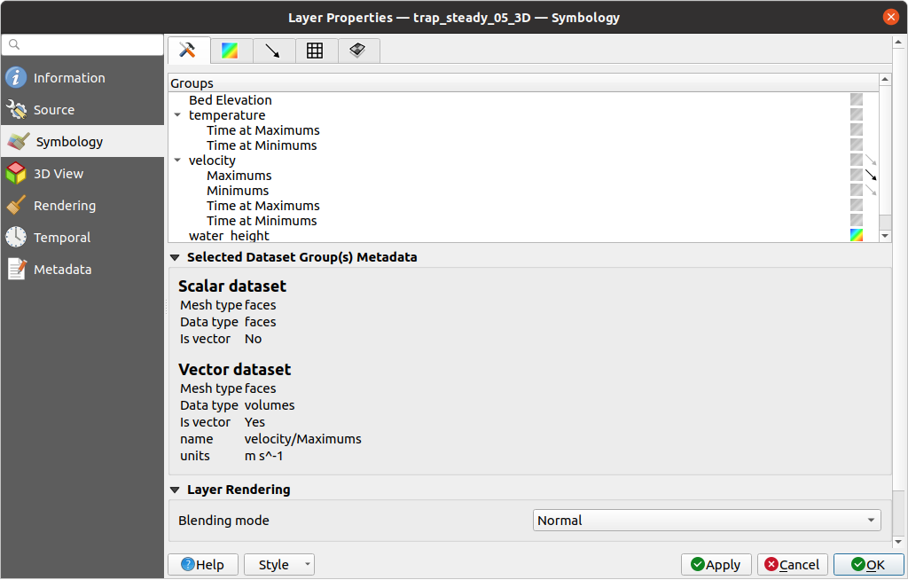
Fig. 17.6 Mesh Layer Datasets

You can apply symbology to the selected vector and/or scalar group using the next tabs.

17.3.3.2. Contours Symbology

Note

The ^Contours tab can be activated only if a scalar dataset has been selected in the Datasets tab.

In the ^Contours tab you can see and change the current visualization options of contours for the selected group, as shown in Fig. 17.7 below:

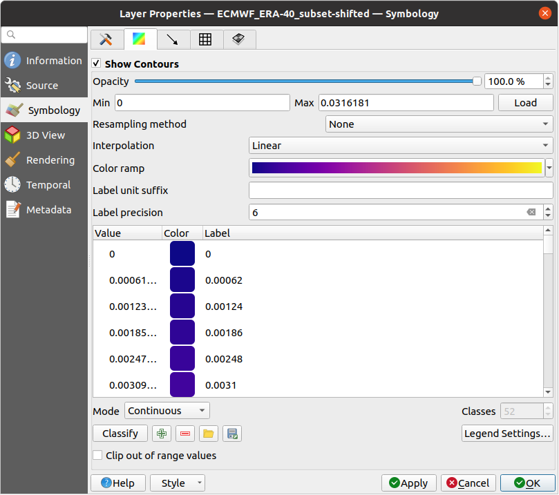
Fig. 17.7 Styling Contours in a Mesh Layer

• For 1D mesh, set the Stroke width of the edges. This can be a fixed size for the whole dataset, or vary along the geometry (more details with the interpolated line renderer)

• Use the slider or the spinbox to set the Opacity of the current group, if of a 2D mesh type.

• Enter the range of values you want to represent on the current group: use ^Load to fetch the min and max values of the current group or enter custom values if you want to exclude some.

• For 2D/3D meshes, select the Resampling method to interpolate the values on the surrounding vertices to the faces (or from the surrounding faces to the vertices) using the Neighbour average method. Depending on whether the dataset is defined on the vertices (respectively on the faces), QGIS defaults this setting to None (respectively Neighbour average) method in order to use values on vertices and keep the default rendering smooth.

• Classify the dataset using the color ramp shader classification.

17.3.3.3. Vectors Symbology

Note

The ^Vectors tab can be activated only if a vector dataset has been selected in the Datasets tab.

In the ^Vectors tab you can see and change the current visualization options of vectors for the selected group, as shown in Fig. 17.8:

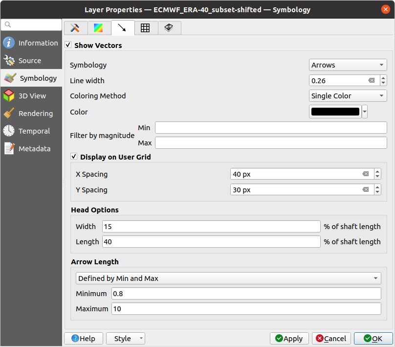
Fig. 17.8 Styling Vectors in a Mesh Layer with arrows

Mesh vector dataset can be styled using various types of Symbology:

• Arrows: vectors are represented with arrows at the same place as they are defined in the raw dataset (i.e. on the nodes or centre of elements) or on a user-defined grid (hence, they are evenly distributed). The arrow length is proportional to the magnitude of the arrow as defined in the raw data but can be scaled by various methods.

• Streamlines: vectors are represented with streamlines seeded from start points. The seeding points can start from the vertices of the mesh, from a user grid or randomly.

• Traces: a nicer animation of the streamlines, the kind of effect you get when you randomly throws sand in the water and see where the sand items flows.

Available properties depend on the selected symbology as shown in the following table.

Label	Description and Properties	Arrow	Streamlines	Traces
Line width	Width of the vector representation
Coloring method	a Single color assigned to all vectors or a variable color based on vectors magnitude, using a Color ramp shader
Filter by magnitude	Only vectors whose length for the selected dataset falls between a Min and Max range are displayed
Display on user grid	Places the vector on a grid with custom X spacing and Y spacing and interpolates their length based on neighbours
Head options	Length and Width of the arrow head, as a percentage of its shaft length
Arrow length	Defined by Min and Max: You specify the minimum and maximum length for the arrows, QGIS will interpolate their size based on the underlying vector’s magnitude Scale to magnitude: arrow length is proportional to their vector’s magnitude Fixed: all the vectors are shown with the same length
Streamlines seeding method	On mesh/grid: relies on the user grid to display the vectors Randomly: vector placement is randomly done with respect to a certain density
Particles count	The amount of “sand” you want to throw into visualisation
Max tail length	The time until the particle fades out

17.3.3.4. Rendering

In the tab ^Rendering tab, QGIS offers possibilities to display and customize the mesh structure. Line width and Line color can be set to represent:

• the edges for 1D meshes

• For 2D meshes:

  • Native mesh rendering: shows original faces and edges from the layer

  • Triangular mesh rendering: adds more edges and displays the faces as triangles

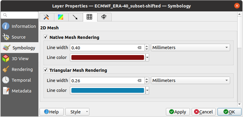
Fig. 17.9 2D Mesh Rendering

17.3.3.5. Stacked mesh averaging method

3D layered meshes consist of multiple stacked 2D unstructured meshes each extruded in the vertical direction (levels) by means of a vertical coordinate. The vertices and faces have the same topology in each vertical level. Values are usually stored on the volumes that are regularly stacked over base 2d mesh. In order to visualise them on 2D canvas, you need to convert values on volumes (3d) to values on faces (2d) that can be shown in mesh layer. The ^{Stacked mesh averaging method} provides different averaging/interpolation methods to handle this.

You can select the method to derive the 2D datasets and corresponding parameters (level index, depth or height values). For each method, an example of application is shown in the dialog but you can read more on the methods at https://fvwiki.tuflow.com/index.php?title=Depth_Averaging_Results.

17.3.4. 3D View Properties

Mesh layers can be used as terrain in a 3D map view based on their vertices Z values. From the 3D properties tab, it’s also possible to render the mesh layer’s dataset in the same 3D view. Therefore, the vertical component of the vertices can be set equal to dataset values (for example, level of water surface) and the texture of the mesh can be set to render other dataset values with color shading (for example velocity).

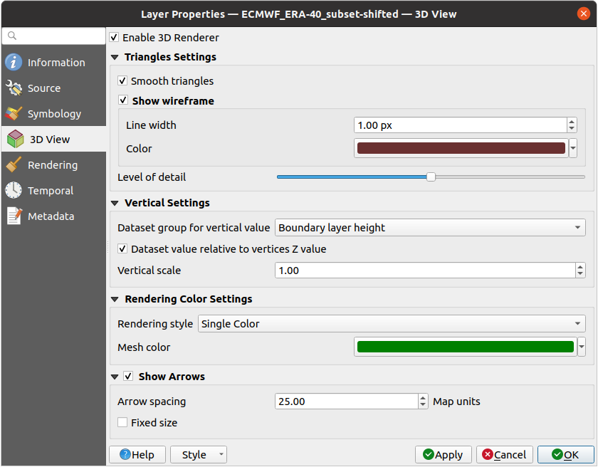
Fig. 17.10 Mesh dataset 3D properties

Check Enable 3D Renderer and you can edit following properties:

• Under Triangle settings

  • Smooth triangles: Angles between consecutive triangles are smoothed for a better 3D rendering

  • Show wireframe whose you can set the Line width and Color

  • Level of detail: Controls how simplified the mesh layer to render should be. On the far right, it is the base mesh, and the more you go left, the more the layer is simplified and is rendered with less details. This option is only available if the Simplify mesh option under the Rendering tab is activated.

• Vertical settings to control behavior of the vertical component

  of vertices of rendered triangles

  • Dataset group for vertical value: the dataset group that will be used for the vertical component of the mesh

  • Dataset value relative to vertices Z value: whether to consider the dataset values as absolute Z coordinate or relative to the vertices native Z value

  • Vertical scale: the scale factor to apply to the dataset Z values

• Rendering color settings with a Rendering style that can be based on the color ramp shader set in Contours Symbology (2D contour color ramp shader) or as a Single color with an associated Mesh color

• Show arrows: displays arrows on mesh layer dataset 3D entity, based on the same vector dataset group used in the vector 2D rendering. They are displayed using the 2D color setting. It’s also possible to define the Arrow spacing and, if it’s of a Fixed size or scaled on magnitude. This spacing setting defines also the max size of arrows because arrows can’t overlap.

17.3.5. Rendering Properties

As mesh layers can have millions of faces, their rendering can sometimes be very slow, especially when all the faces are displayed in the view whereas they are too small to be viewed. To speed up the rendering, you can simplify the mesh layer, resulting in one or more meshes representing different levels of detail and select at which level of detail you would like QGIS to render the mesh layer. Note that the simplify mesh contains only triangular faces.

From the Rendering tab, check Simplify mesh and set:

• a Reduction factor: Controls generation of successive levels of simplified meshes. For example, if the base mesh has 5M faces, and the reduction factor is 10, the first simplified mesh will have approximately 500 000 faces, the second 50 000 faces, the third 5000,… If a higher reduction factor leads quickly to simpler meshes (i.e. with triangles of bigger size), it produces also fewer levels of detail.

• Minimum triangle size: the average size (in pixels) of the triangles that is permitted to display. If the average size of the mesh is lesser than this value, the rendering of a lower level of details mesh is triggered.

17.3.6. Temporal Properties

The Temporal tab provides options to control the rendering of the layer over time. It allows to dynamically display temporal values of the enabled dataset groups. Such a dynamic rendering requires the temporal navigation to be enabled over the map canvas.

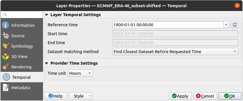
Fig. 17.11 Mesh Temporal properties

Layer temporal settings

• Reference time of the dataset group, as an absolute date time. By default, QGIS parses the source layer and returns the first valid reference time in the layer’s dataset group. If unavailable, the value will be set by the project time range or fell back to the current date. The Start time and End time to consider are then calculated based on the internal timestamp step of the dataset.

  It is possible to set a custom Reference time (and then the time range), and revert the changes using the ^{Reload from provider} button.

• Dataset matching method: determines the dataset to display at the given time. Options are Find closest dataset before requested time or Find closest dataset from requested time (after or before).

Provider time settings

• Time unit extracted from the raw data, or user defined. This can be used to align the speed of the mesh layer with other layers in the project during map time navigation. Supported units are Seconds, Minutes, Hours and Days.

17.3.7. Metadata Properties

The Metadata tab provides you with options to create and edit a metadata report on your layer. See Metadata for more information.

17.4. Mesh Calculator

The Mesh Calculator tool from the top Mesh menu allows you to perform arithmetic and logical calculations on existing dataset groups to generate a new dataset group (see Fig. 17.12).

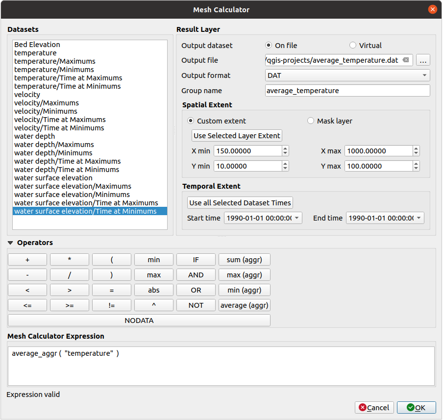
Fig. 17.12 Mesh Calculator

The Datasets list contains all dataset groups in the active mesh layer. To use a dataset group in an expression, double click its name in the list and it will be added to the Mesh calculator expression field. You can then use the operators to construct calculation expressions, or you can just type them into the box.

The Result Layer helps you configure properties of the output layer:

• Create on-the-fly dataset group instead of writing layer to disk:

  • If unchecked, the output is stored on disk as a new plain file. An Output File path and an Output Format are required.

  • If checked, a new dataset group will be added to the mesh layer. Values of the dataset group are not stored in memory but each dataset is calculated when needed with the formula entered in the mesh calculator. That virtual dataset group is saved with the project, and if needed, it can be removed or made persistent in file from the layer Source properties tab.

  In either case, you should provide a Group Name for the output dataset group.

• The Spatial extent to consider for calculation can be:

  • a Custom extent, manually filled with the X min, X max, Y min and Y max coordinate, or extracted from an existing dataset group (select it in the list and press Use selected layer extent to fill the abovementioned coordinate fields)

  • defined by a polygon layer (Mask layer) of the project: the polygon features geometry are used to clip the mesh layer datasets

• The Temporal extent to take into account for datasets can be set with the Start time and End time options, selected from the existing dataset groups timesteps. They can also be filled using the Use all selected dataset times button to take the whole range.

The Operators section contains all available operators. To add an operator to the raster calculator expression box, click the appropriate button. Mathematical calculations (+, -, *, … ) and statistical functions (min, max, sum (aggr), average (aggr), … ) are available. Conditional expressions (=, !=, <, >=, IF, AND, NOT, … ) return either 0 for false and 1 for true, and therefore can be used with other operators and functions. The NODATA value can also be used in the expressions.

The Mesh Calculator Expression widget shows and lets you edit the expression to execute.