20. 回答シート
20.1. Results For 最初のレイヤを追加
20.2. Results For インタフェースのあらまし
20.2.1.  あらまし (パート 1)
Refer back to the image showing the interface layout and check that you remember the names and functions of the screen elements.
20.3. Results For ベクターデータで作業
20.4. Results For Symbology
20.4.1. 色
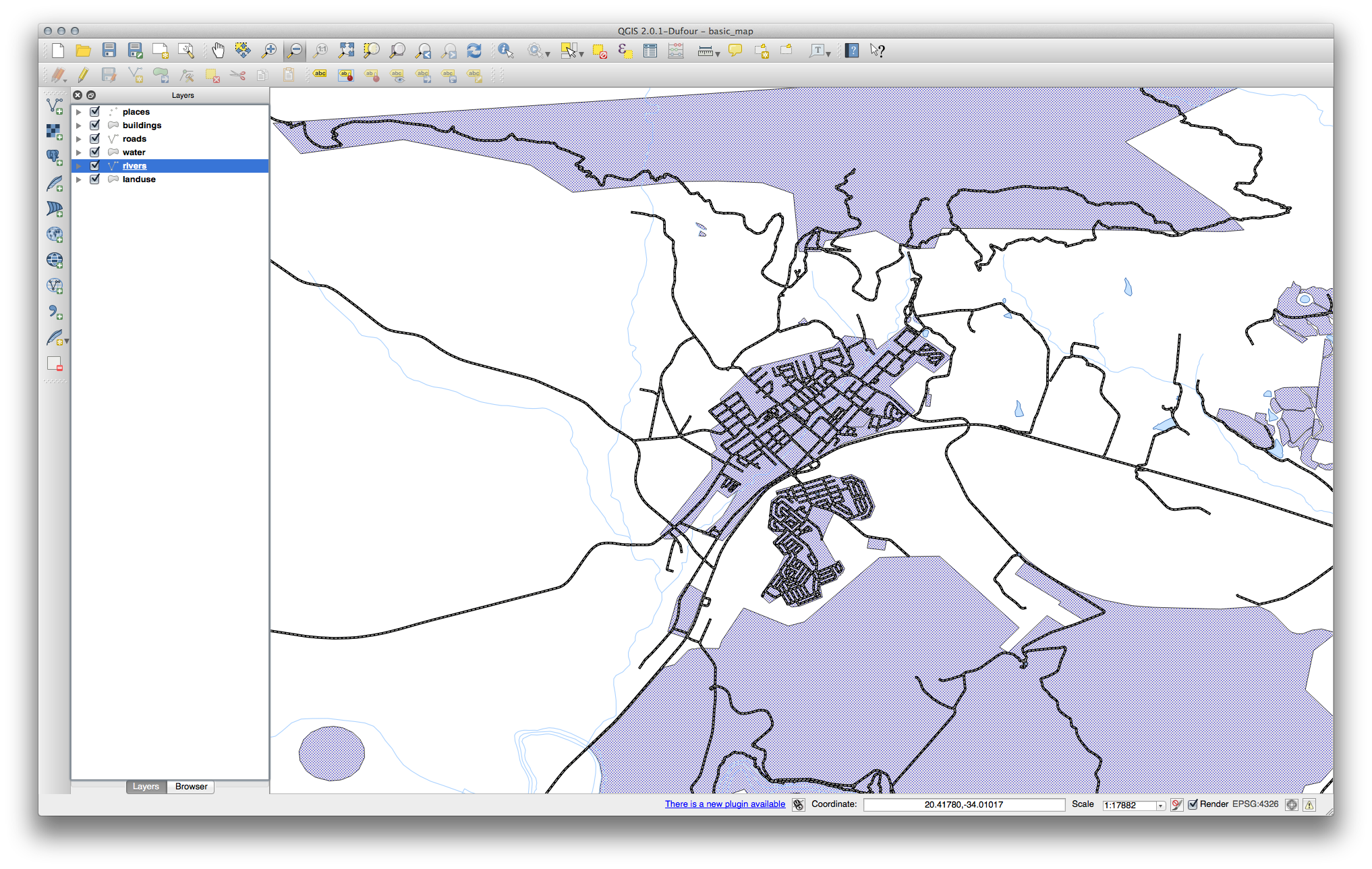
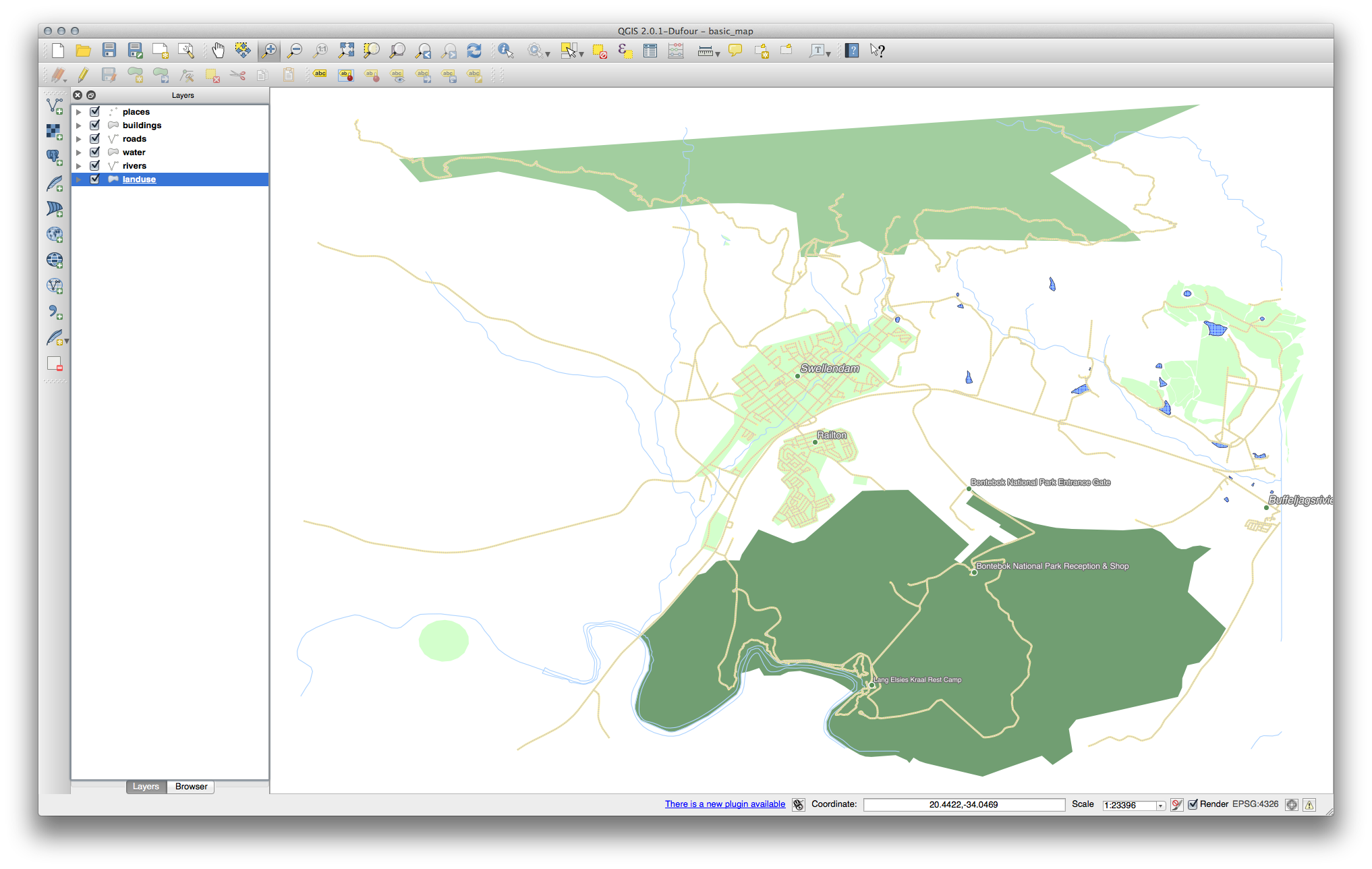
色が期待通りに変わっているか確認してください。
現時点では 水系 レイヤを変えるだけで十分です。下記はその例ですが、選んだ色によっては違って見えるかもしれません。
ノート
他のレイヤに煩わされずに一度にひとつのレイヤだけで作業したい場合、レイヤ一覧内のその名前の隣にあるチェックボックス内をクリックしてレイヤを非表示にできます。ボックスが空の場合にレイヤは非表示です。
20.4.2. シンボルの構造
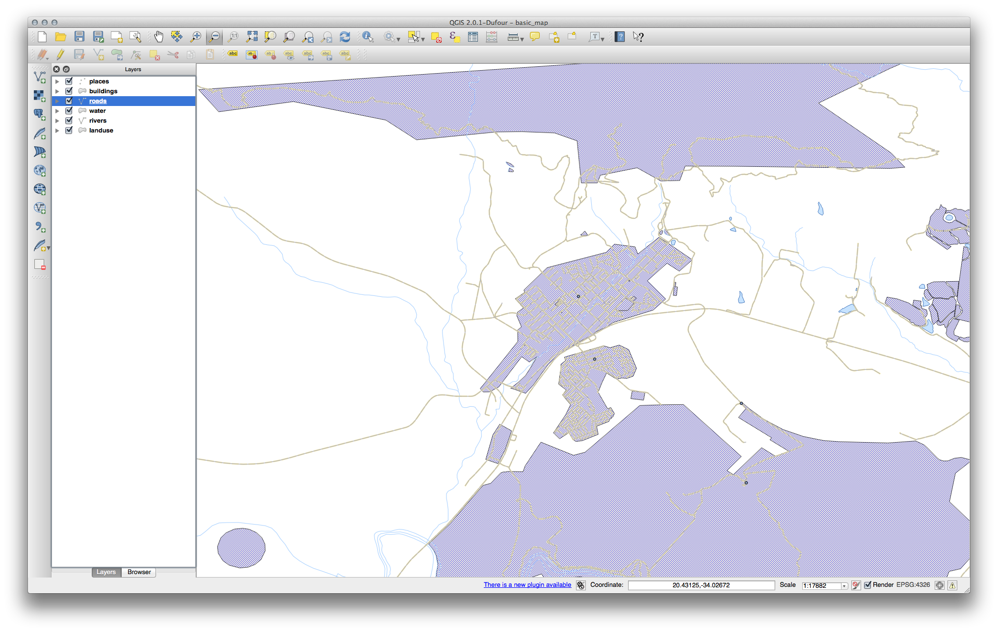
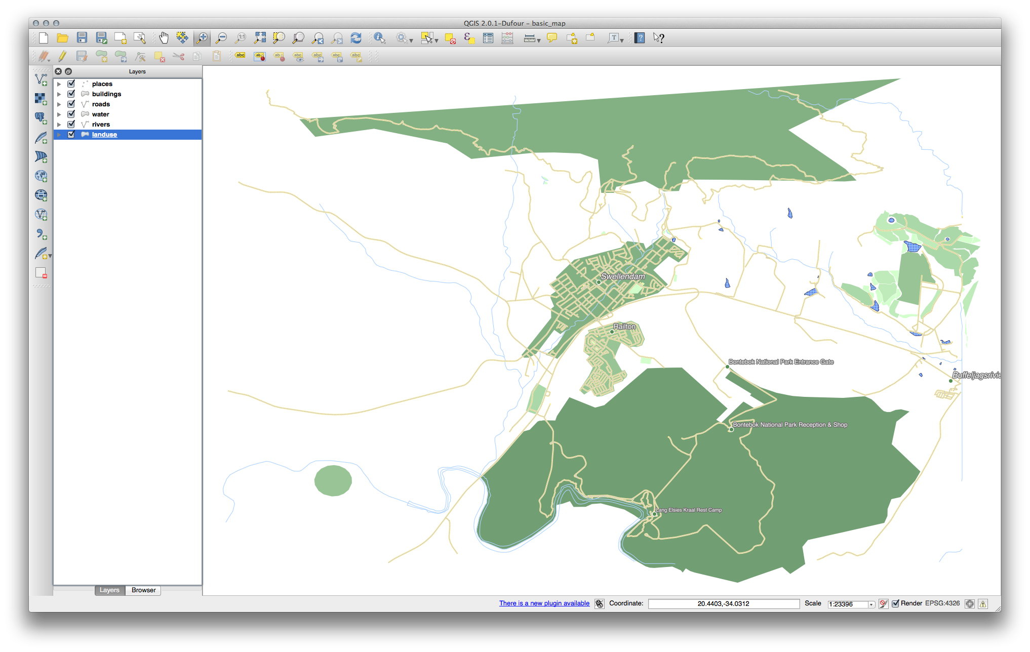
これであなたのマップはこのように見えていると思います:
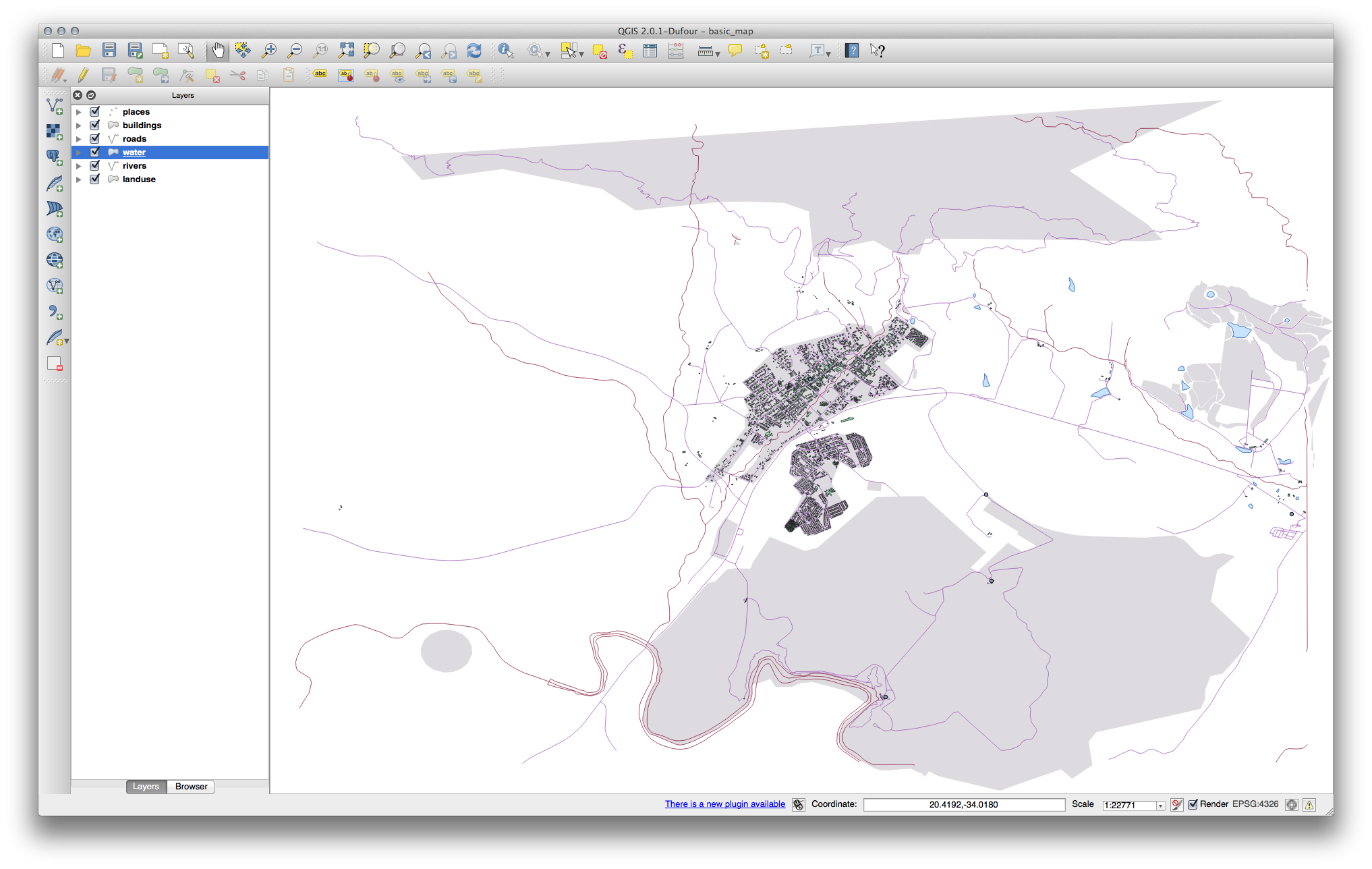
あなたが初心者レベルのユーザであれば、ここで止めた方が良いかもしれません。
上のメソッドを使って残りのレイヤすべての色とスタイルを変更します。
オブジェクトにはできるだけ本来の色を使うようにしてください。たとえば、道路は赤や青ではなく、グレイまたは黒であるべきです。
- Also feel free to experiment with different Fill Style and Border Style settings for the polygons.
20.4.4.  シンボルのレベル
必要なシンボルを作るには2つのシンボルレイヤが必要です:
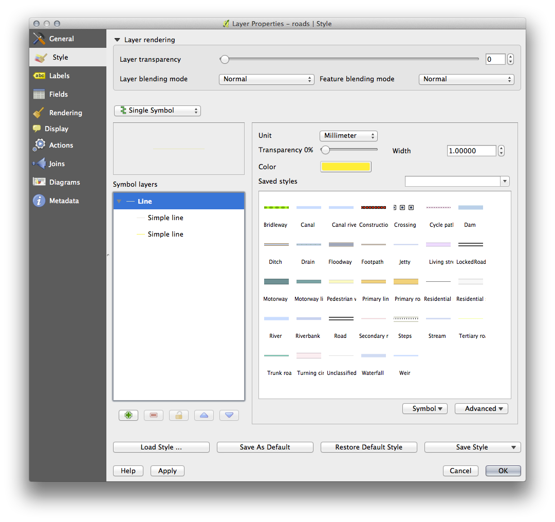
いちばん下のシンボルレイヤは幅広の黄色の実線です。その先頭にはやや狭いグレーの実線があります。
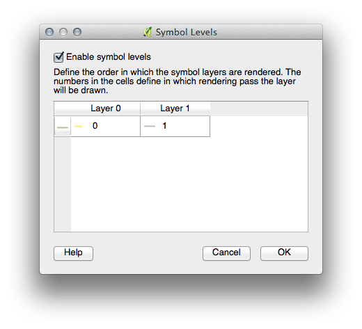
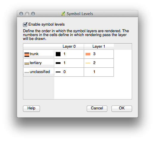
もしあなたのシンボルレイヤが上記に似てはいるが欲しい結果が得られていない場合は、あなたのシンボルレベルが次のように見えるかどうかチェックしてください:
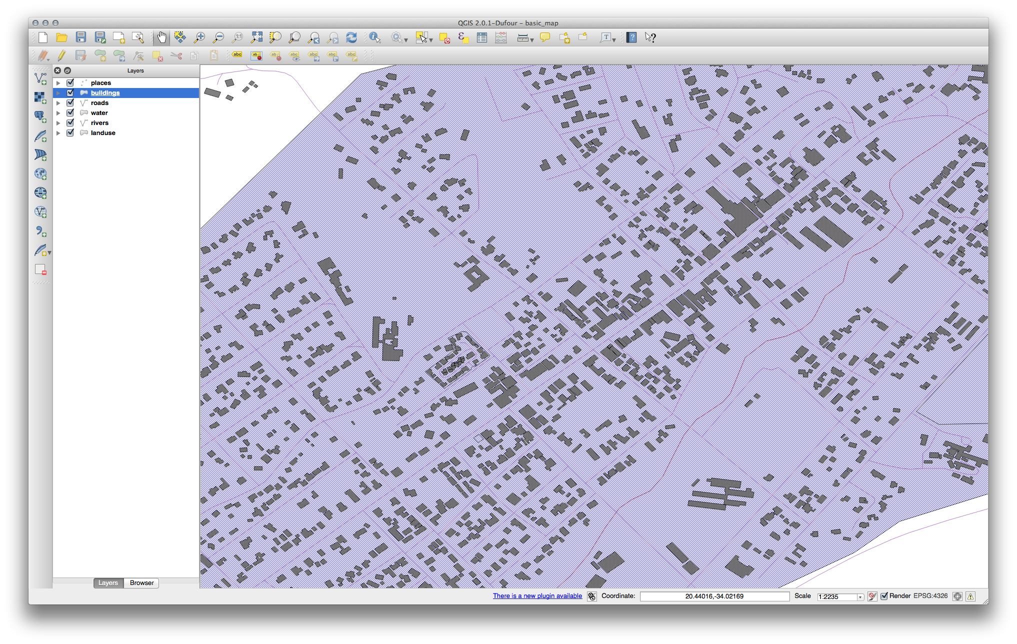
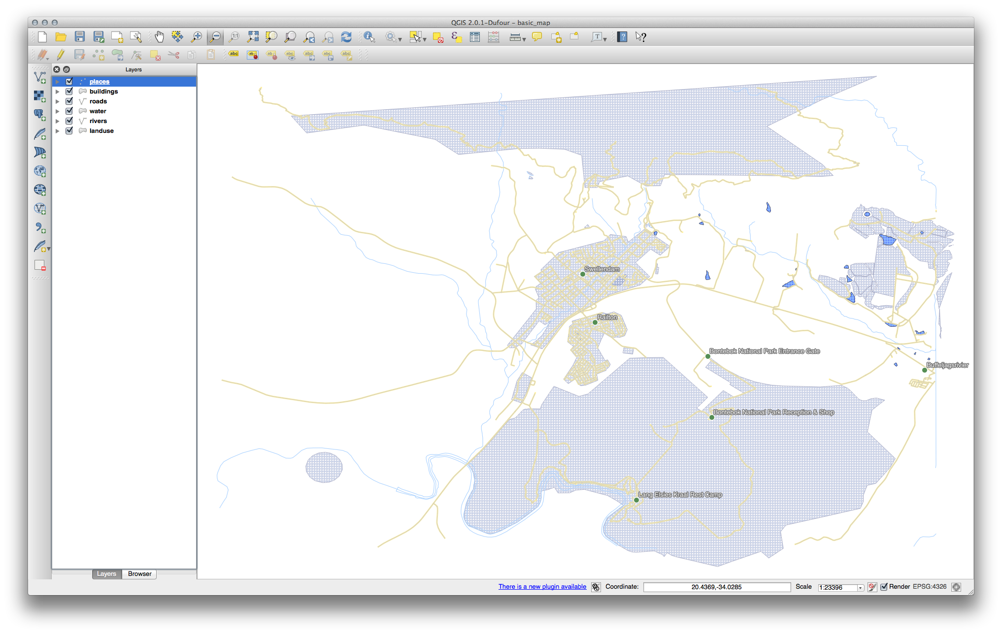
これであなたのマップは次のように見えるようになったはずです:
20.5. Results For 属性データ
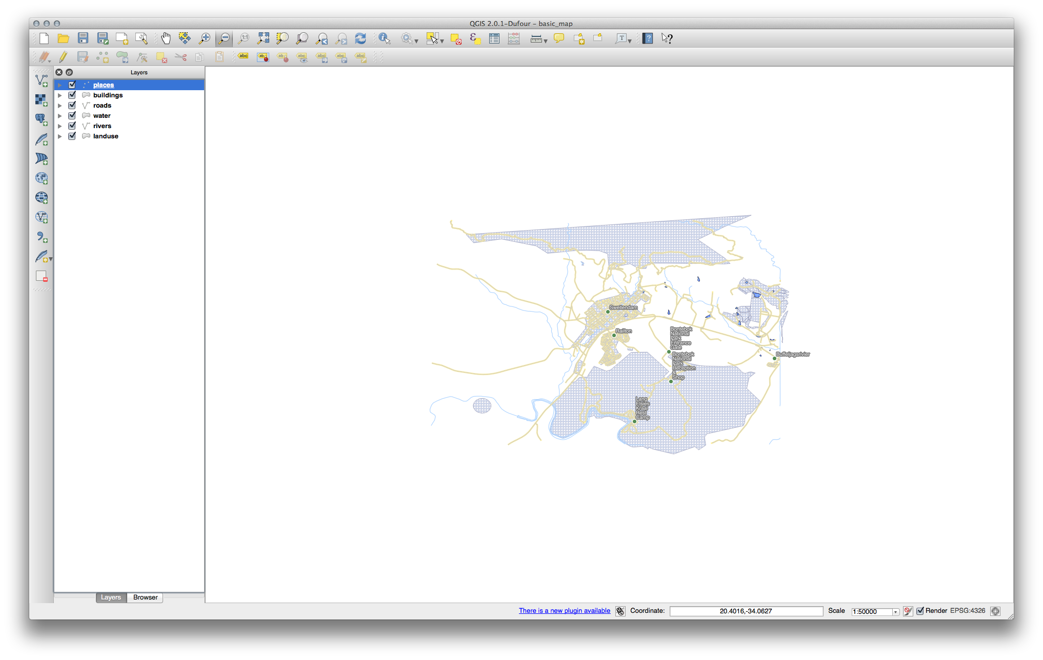
20.6. Results For ラベルツール
20.6.1. ラベルのカスタマイズ (パート 1)
Your map should now show the marker points and the labels should be offset by 2.0 mm: The style of the markers and labels should allow both to be clearly visible on the map:
20.6.2. ラベルのカスタマイズ (パート 2)
One possible solution has this final product:
To arrive at this result:
Use a font size of 10, a Label distance of 1,5 mm, Symbol width and Symbol size of 3.0 mm.
In addition, this example uses the Wrap label on character option:
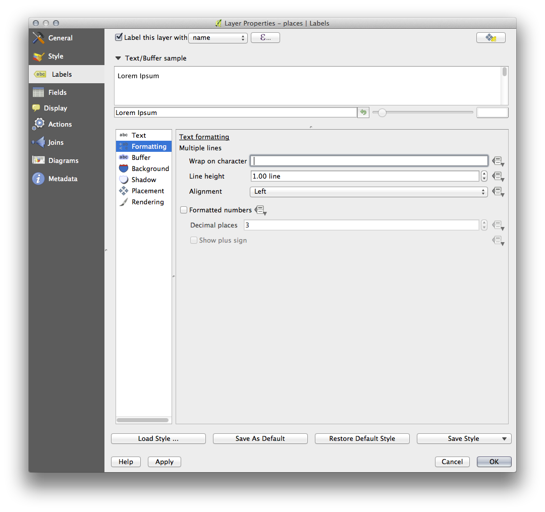
Enter a space in this field and click Apply to achieve the same effect. In our case, some of the place names are very long, resulting in names with multiple lines which is not very user friendly. You might find this setting to be more appropriate for your map.
20.6.3.  Using Data Defined Settings
Still in edit mode, set the FONT_SIZE values to whatever you prefer. The example uses 16 for towns, 14 for suburbs, 12 for localities and 10 for hamlets.
編集モードを抜ける前に忘れずに変更を保存してください。
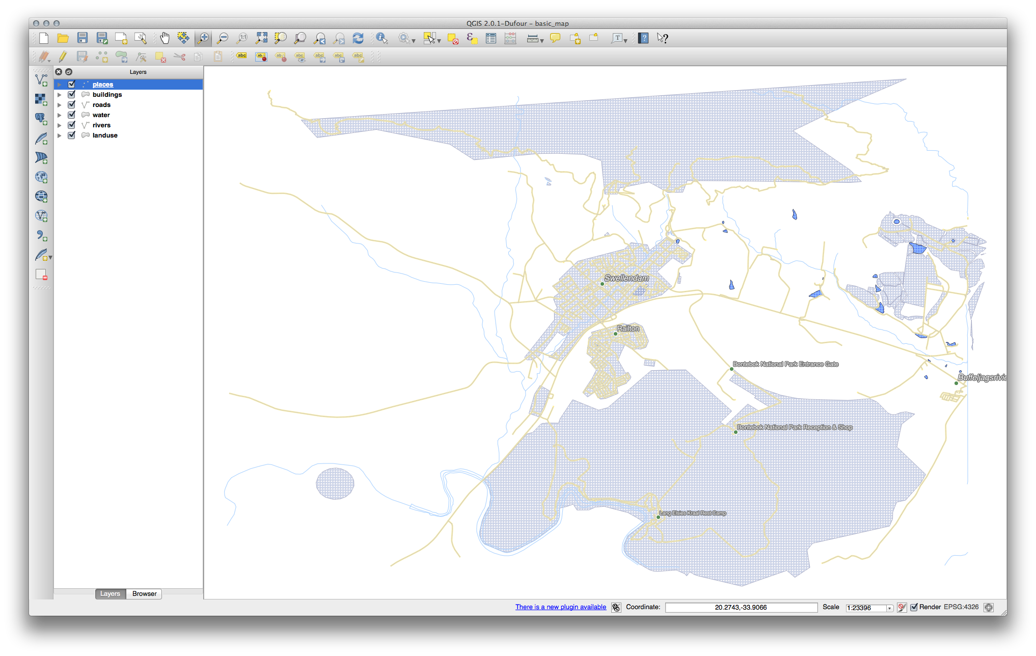
Return to the Text formatting options for the places layer and select FONT_SIZE in the Attribute field of the font size data override dropdown:
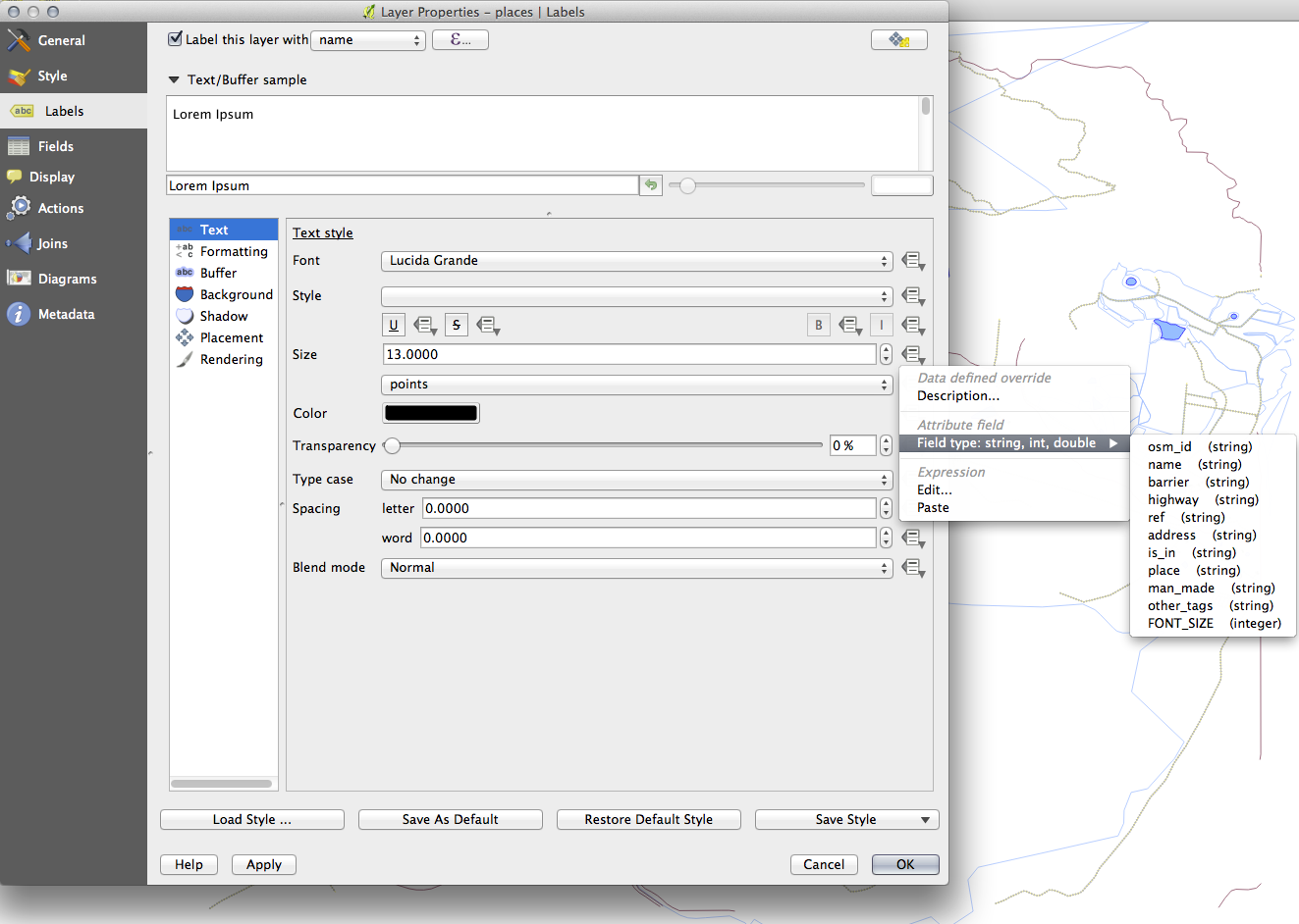
Your results, if using the above values, should be this:
20.7. Results For 分類
20.8. Results For 新しいベクターデータセットの作成
20.8.2. トポロジー: リングツールを追加
正確な形状は重要ではありませんが、あなたの地物の中央には穴が空くことになります。こちらのように。
- Undo your edit before continuing with the exercise for the next tool.
20.8.3. Topology: パートツールを追加
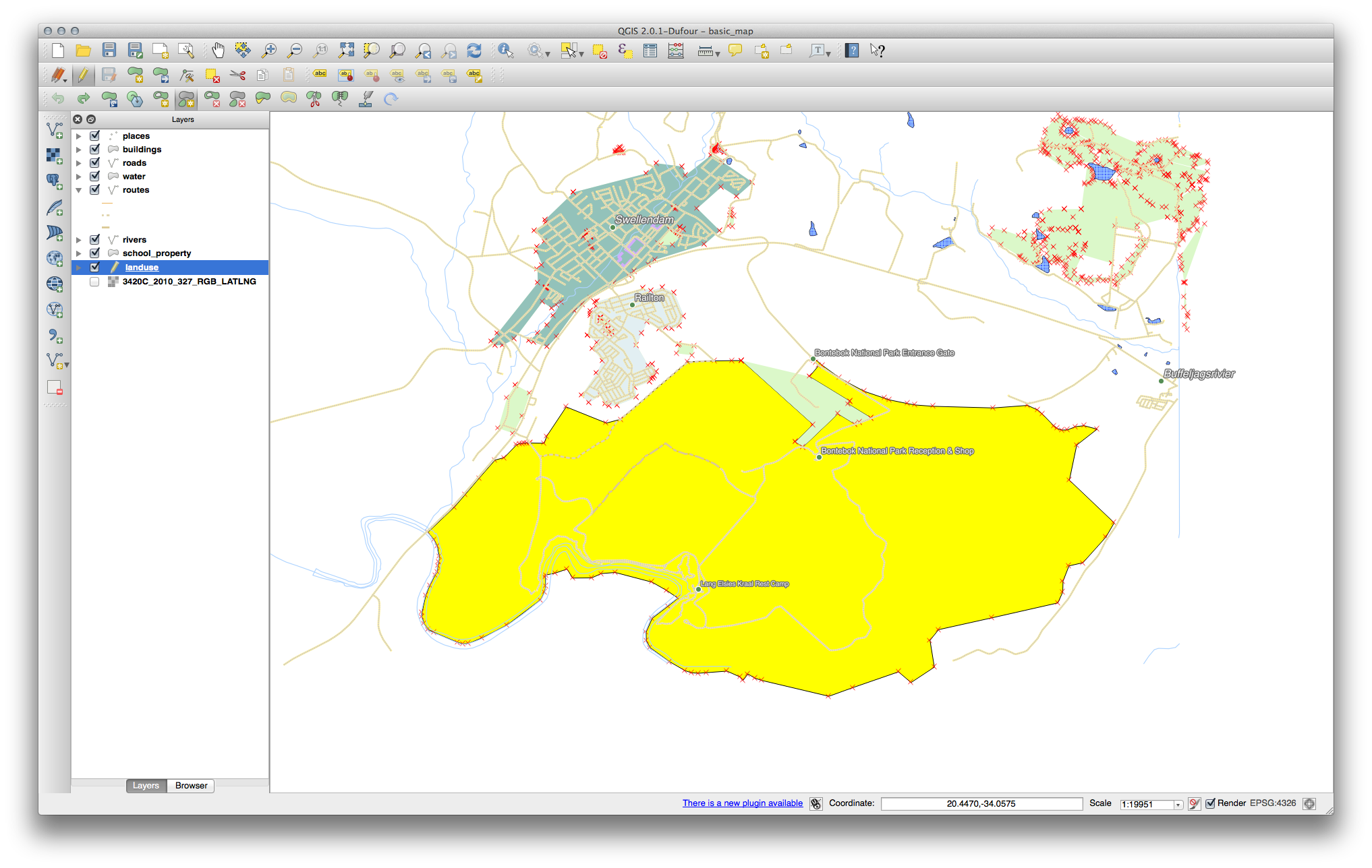
最初に Bontebok National Park を選択します:
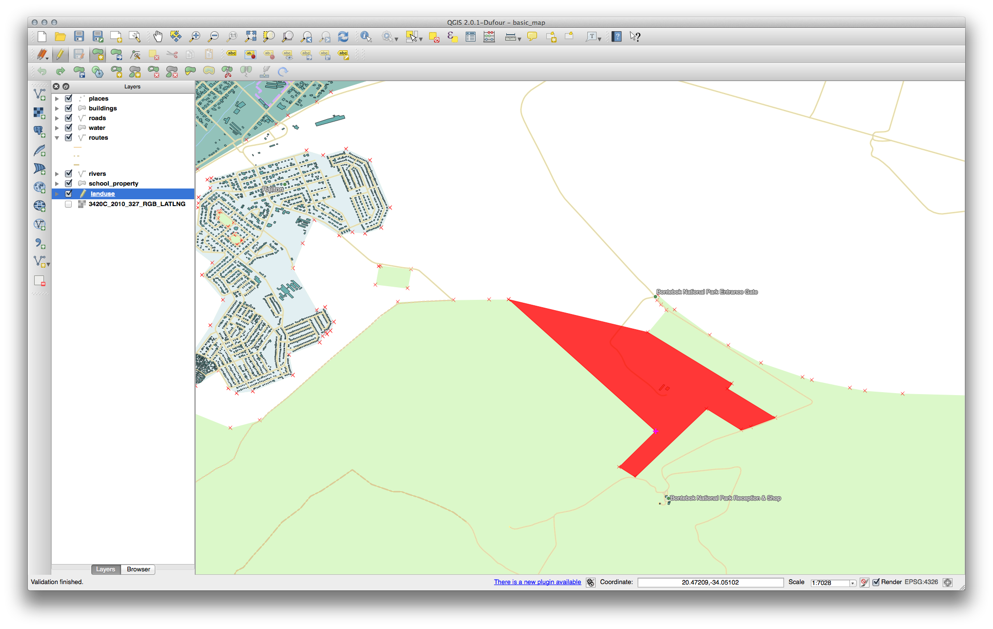
新しいパートを追加:
- Undo your edit before continuing with the exercise for the next tool.
20.8.4. 地物をマージ
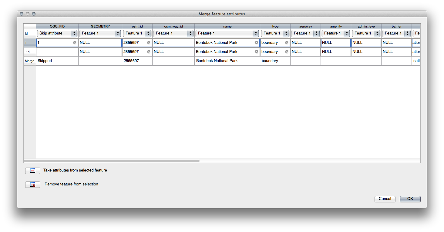
選択した地物のマージ ツールを使う際には、最初にマージしたいポリゴンを両方選んでください。
- Use the feature with the OGC_FID of 1 as the source of your attributes (click on its entry in the dialog, then click the Take attributes from selected feature button):
ノート
- If you’re using a different dataset, it is highly likely that your
- original polygon’s OGC_FID will not be 1. Just choose the feature which has an OGC_FID.
ノート
Using the Merge Attributes of Selected Features tool will keep the geometries distinct, but give them the same attributes.
20.8.5. フォーム
For the TYPE, there is obviously a limited amount of types that a road can be, and if you check the attribute table for this layer, you’ll see that they are predefined.
ウィジェットを バリューマップ にセットして :guilabel:` レイヤからデータをロード` をクリックしてください。
Select roads in the Label dropdown and highway for both the Value and Description options:
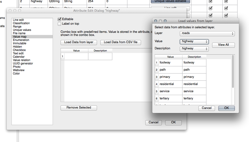
Ok を3回クリックしてください。
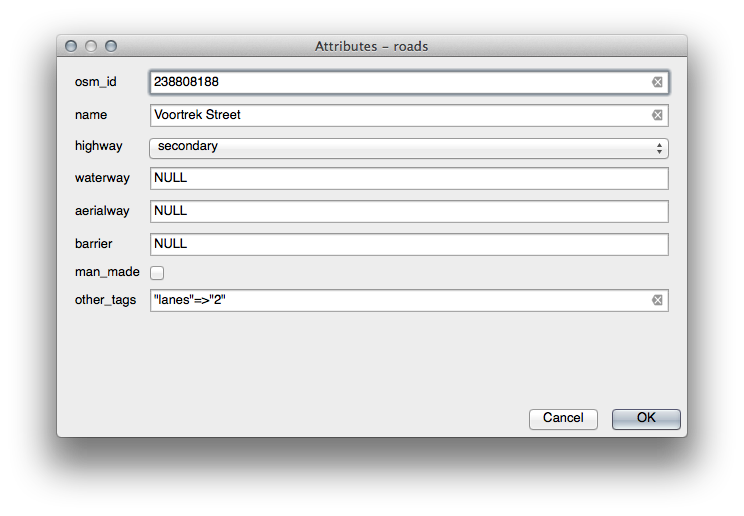
If you use the Identify tool on a street now while edit mode is active, the dialog you get should look like this:
20.9. Results For ベクター分析
20.9.1. OSM データから自分用のレイヤを抽出
For the purpose of this exercise, the OSM layers which we are interested in are multipolygons and lines. The multipolygons layer contains the data we need in order to produce the houses, schools and restaurants layers. The lines layer contains the roads dataset.
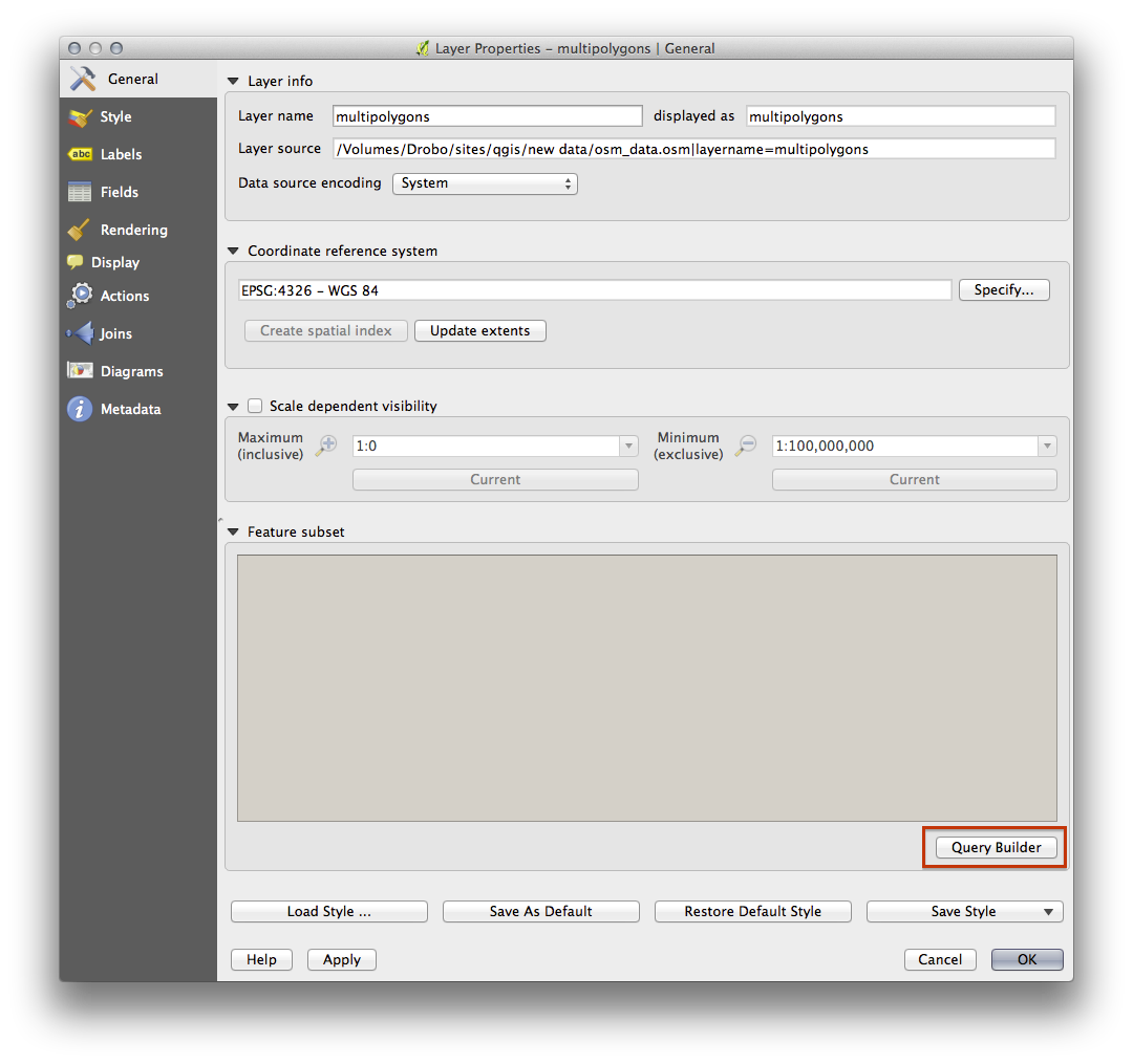
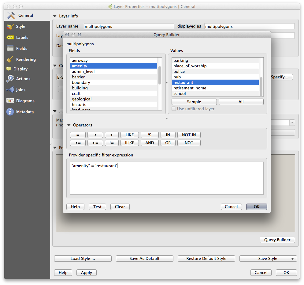
クエリビルダー はレイヤプロパティにあります:
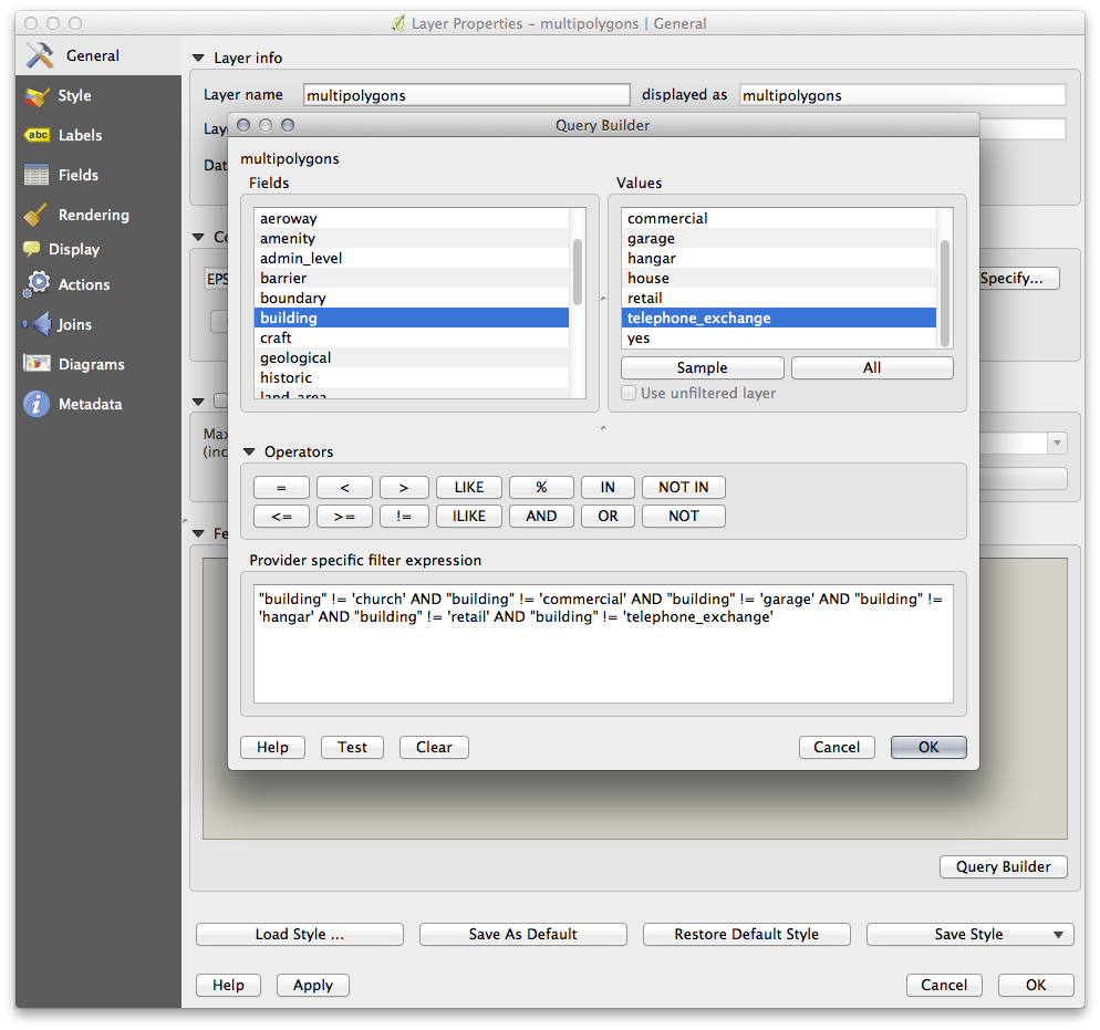
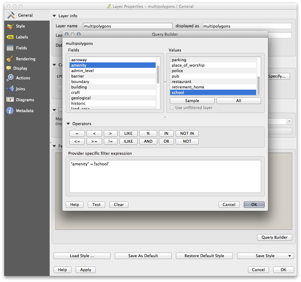
Using the Query Builder against the multipolygons layer, create the following queries for the houses, schools, restaurants and residential layers:
Once you have entered each query, click OK. You’ll see that the map updates to show only the data you have selected. Since you need to use again the multipolygons data from the OSM dataset, at this point, you can use one of the following methods:
- Rename the filtered OSM layer and re-import the layer from osm_data.osm, OR
- Duplicate the filtered layer, rename the copy, clear the query and create your new query in the Query Builder.
ノート
Although OSM’s building field has a house value, the coverage in your area - as in ours - may not be complete. In our test region, it is therefore more accurate to exclude all buildings which are defined as anything other than house. You may decide to simply include buildings which are defined as house and all other values that have not a clear meaning like yes.
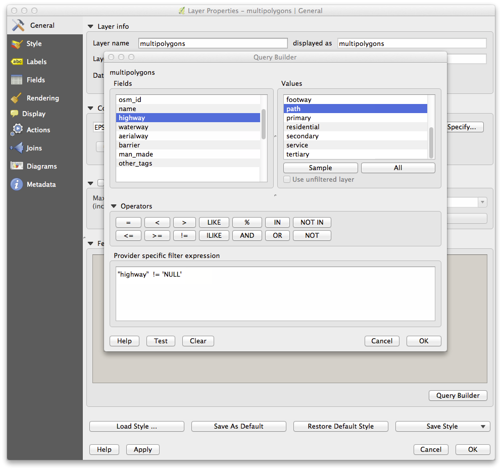
To create the roads layer, build this query against OSM’s lines layer:
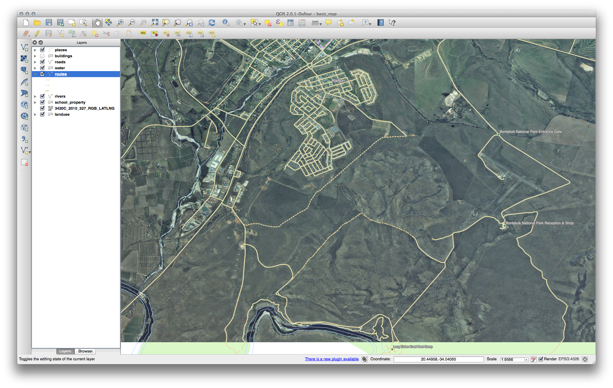
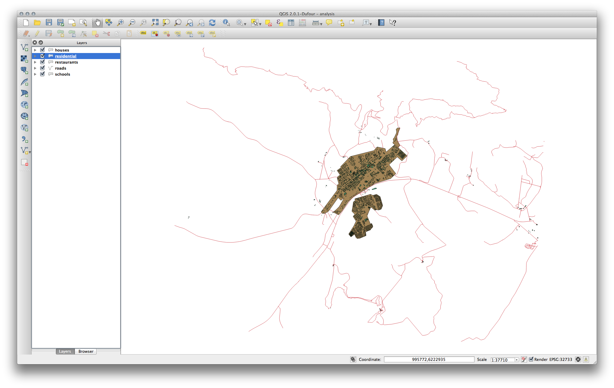
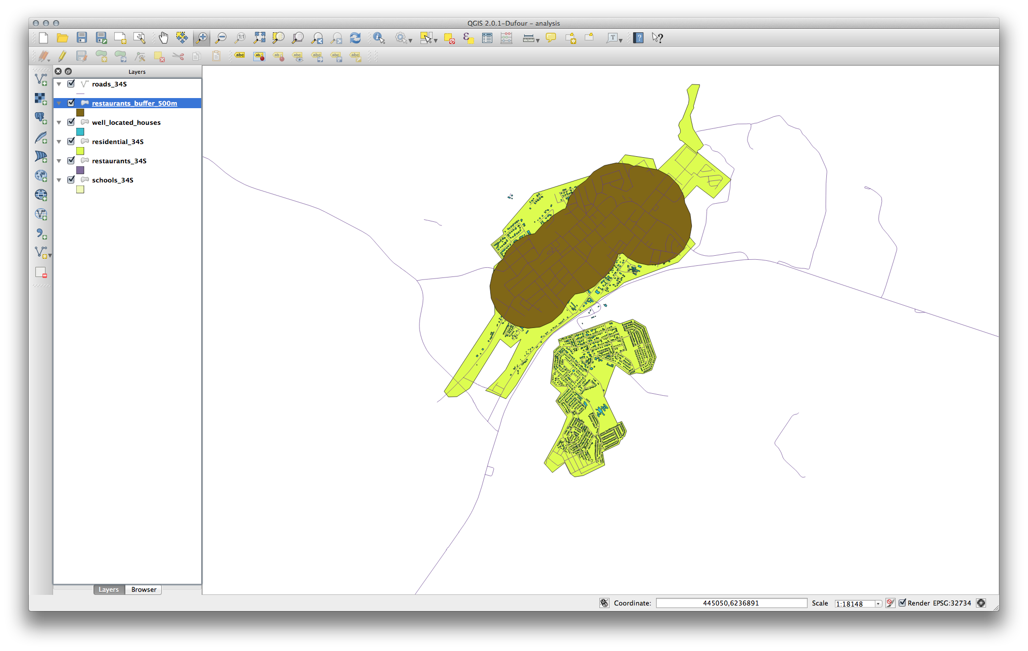
You should end up with a map which looks similar to the following:
20.9.2. 高校からの距離
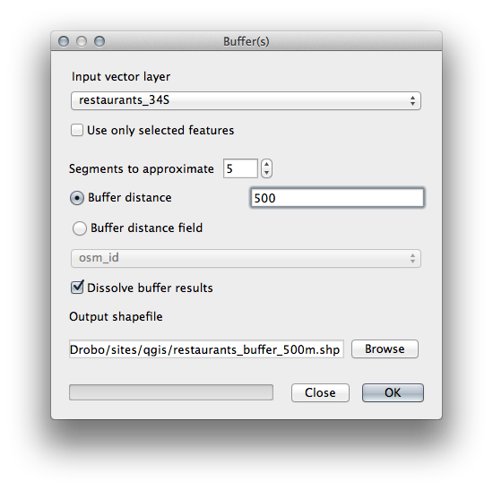
あなたのバッファダイアログはこのように見えるはずです:
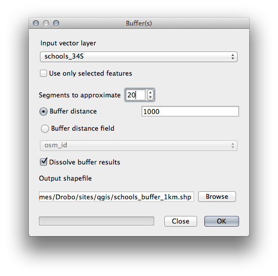
バッファ距離 は 1000 メーターです (すなわち 1 キロメーター)。
The Segments to approximate value is set to 20. This is optional, but it’s recommended, because it makes the output buffers look smoother. Compare this:
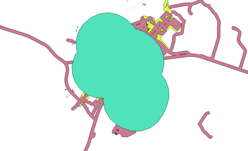
To this:
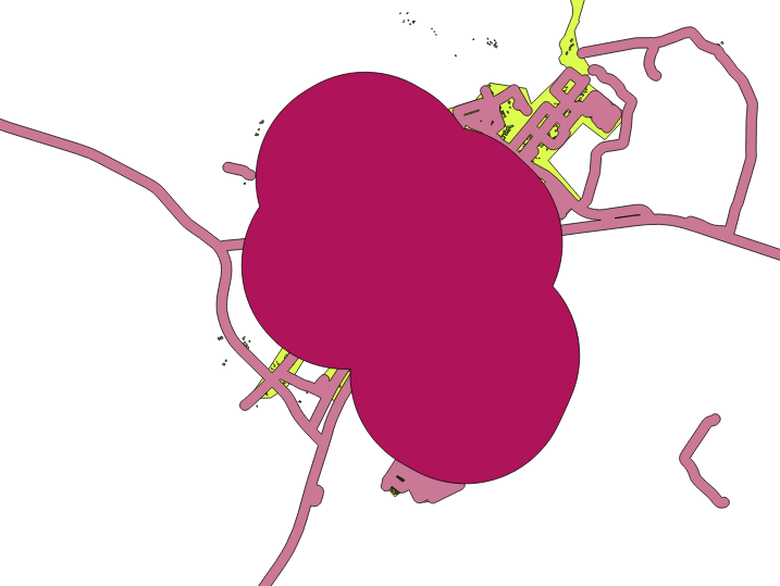
The first image shows the buffer with the Segments to approximate value set to 5 and the second shows the value set to 20. In our example, the difference is subtle, but you can see that the buffer’s edges are smoother with the higher value.
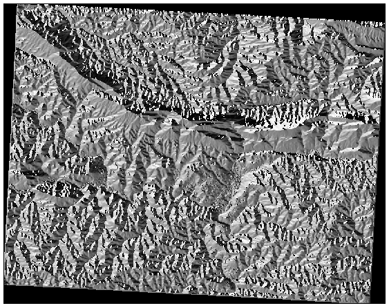
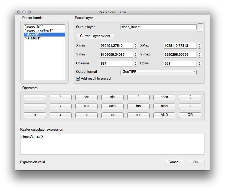
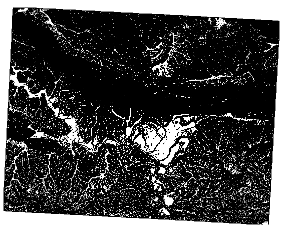
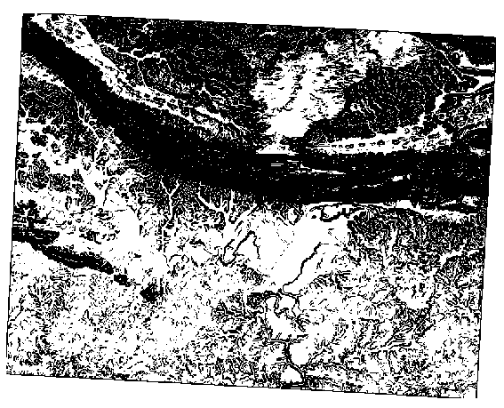
20.10. Results For ラスタ分析
20.11. Results For 分析を完了させる
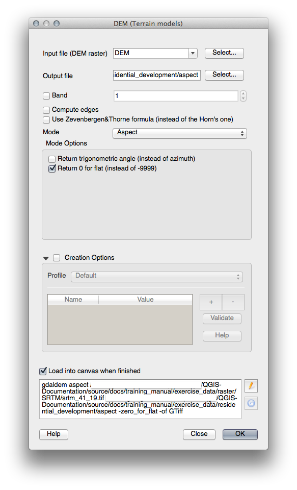
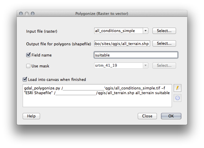
20.11.1. ラスタからベクタ
- Open the Query Builder by right-clicking on the all_terrain layer in the Layers list, select the General tab.
- Then build the query "suitable" = 1.
- Click OK to filter out all the polygons where this condition isn’t met.
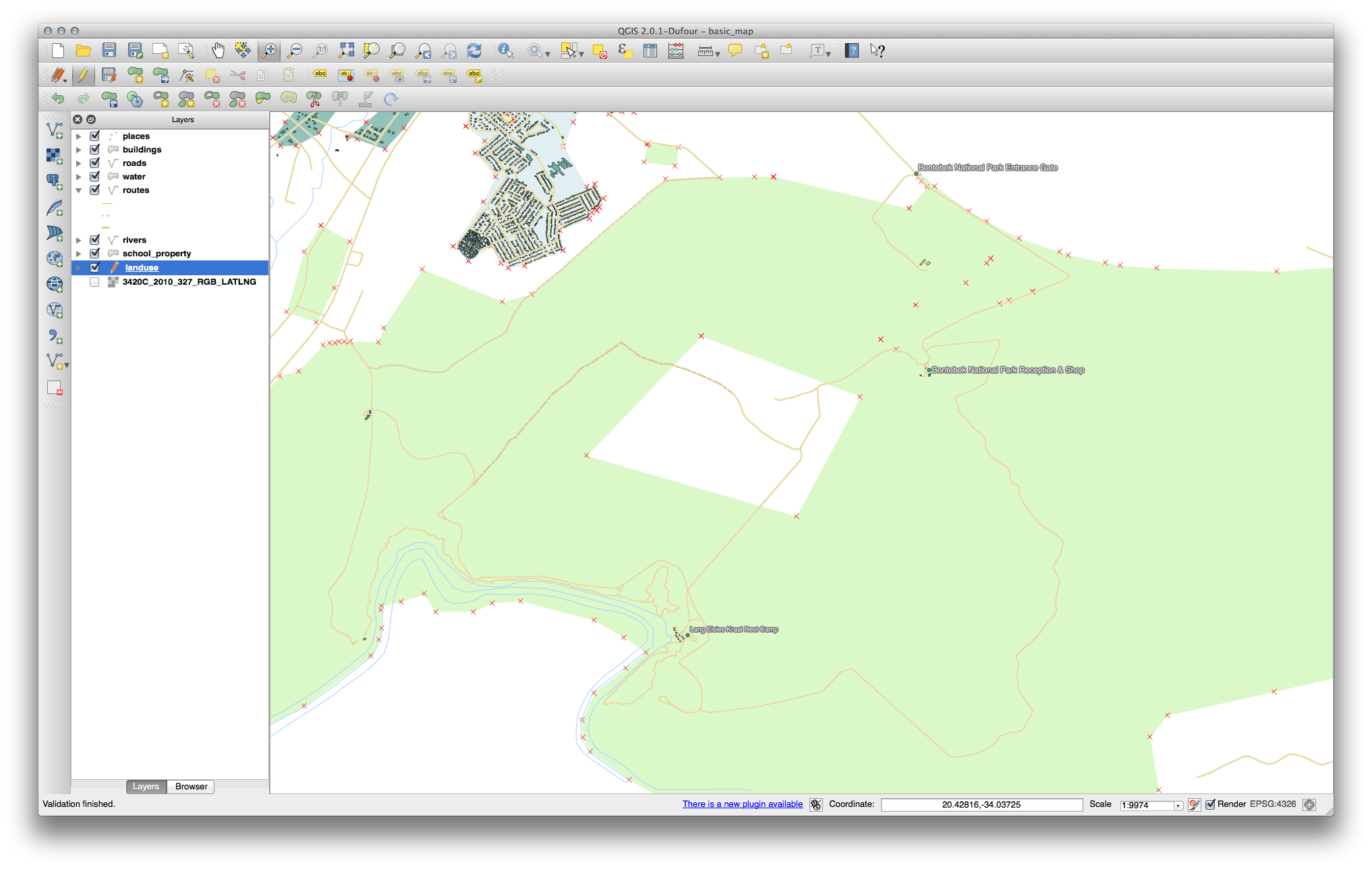
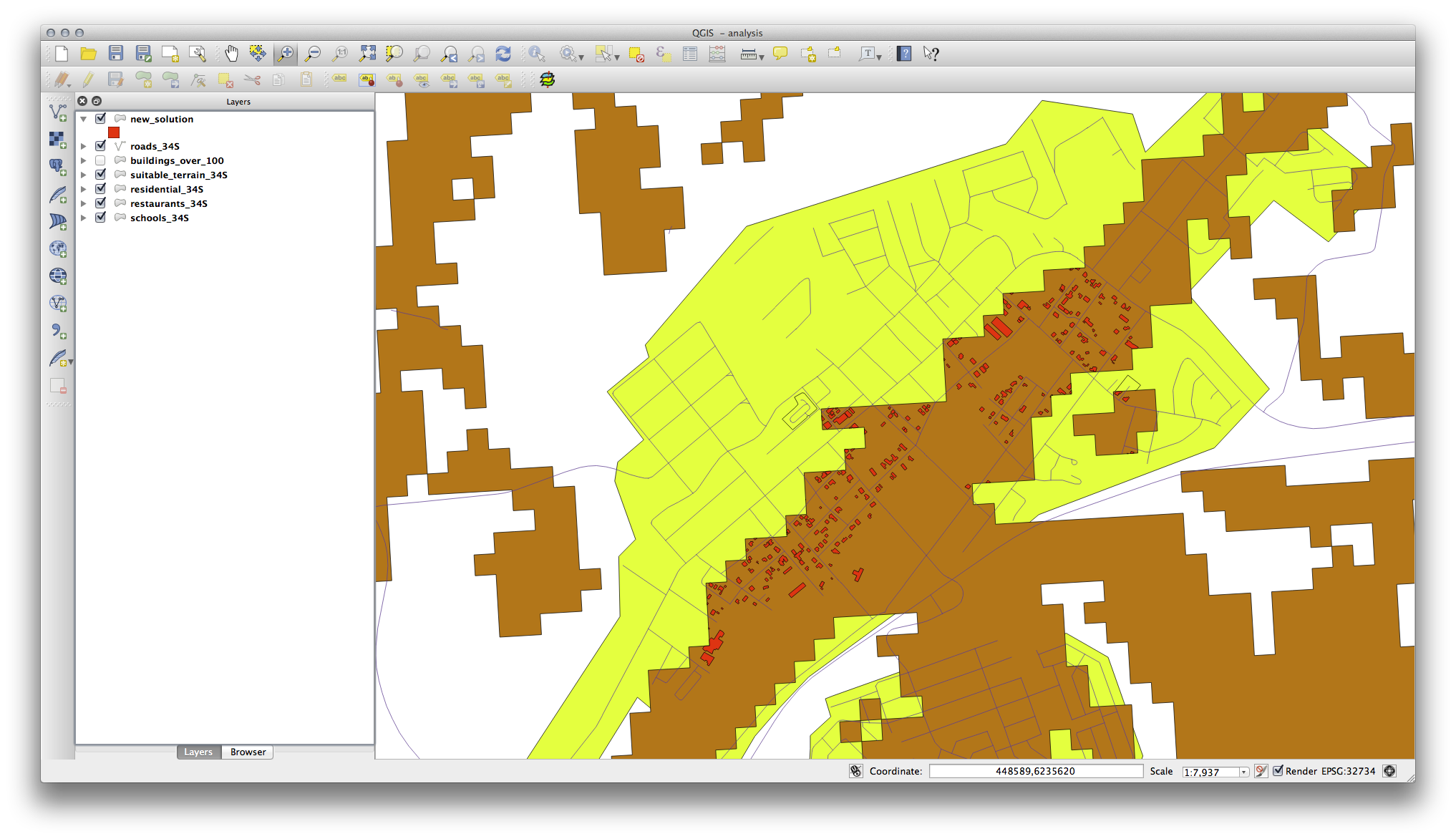
オリジナルのラスタ上で閲覧するとその領域は完全にオーバーラップされるはずです:
- You can save this layer by right-clicking on the all_terrain layer in the Layers list and choosing Save As..., then continue as per the instructions.
20.11.2. 結果を精査
You may notice that some of the buildings in your new_solution layer have been “sliced” by the Intersect tool. This shows that only part of the building - and therefore only part of the property - lies on suitable terrain. We can therefore sensibly eliminate those buildings from our dataset
20.11.3. 分析を改善する
現時点ではあなたの分析は次のように見えるはずです:
Consider a circular area, continuous for 100 meters in all directions.
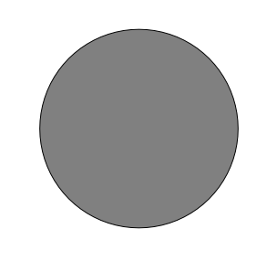
If it is greater than 100 meters in radius, then subtracting 100 meters from its size (from all directions) will result in a part of it being left in the middle.
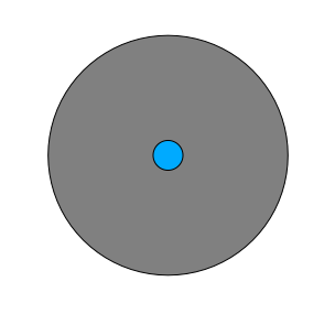
Therefore, you can run an interior buffer of 100 meters on your existing suitable_terrain vector layer. In the output of the buffer function, whatever remains of the original layer will represent areas where there is suitable terrain for 100 meters beyond.
To demonstrate:
Go to Vector ‣ Geoprocessing Tools ‣ Buffer(s) to open the Buffer(s) dialog.
このようにセットアップします:
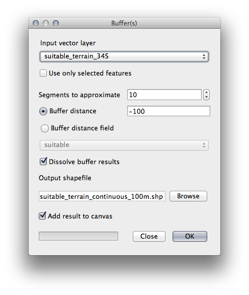
Use the suitable_terrain layer with 10 segments and a buffer distance of -100. (The distance is automatically in meters because your map is using a projected CRS.)
Save the output in exercise_data/residential_development/ as suitable_terrain_continuous100m.shp.
必要に応じて、あなたのオリジナルの suitable_terrain レイヤの上に新しいレイヤを移動してください。
作業結果は次のように見えるはずです:

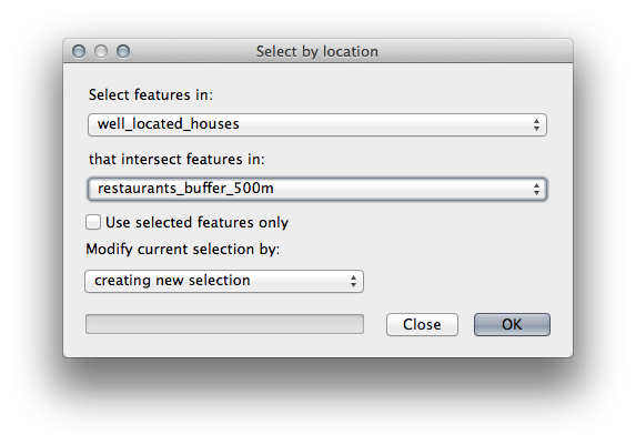
Now use the Select by Location tool (Vector ‣ Research Tools ‣ Select by location).
このようにセットアップします:
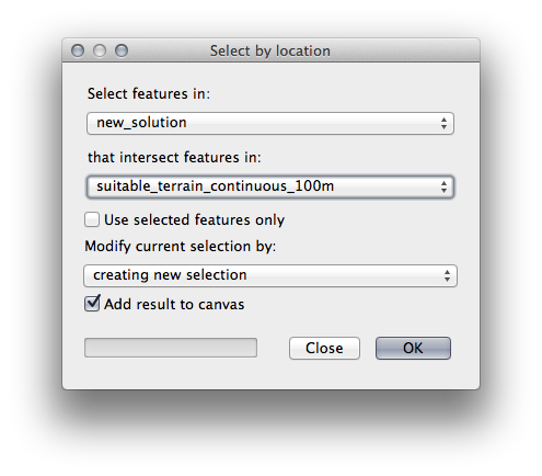
Select features in new_solution that intersect features in suitable_terrain_continuous100m.shp.
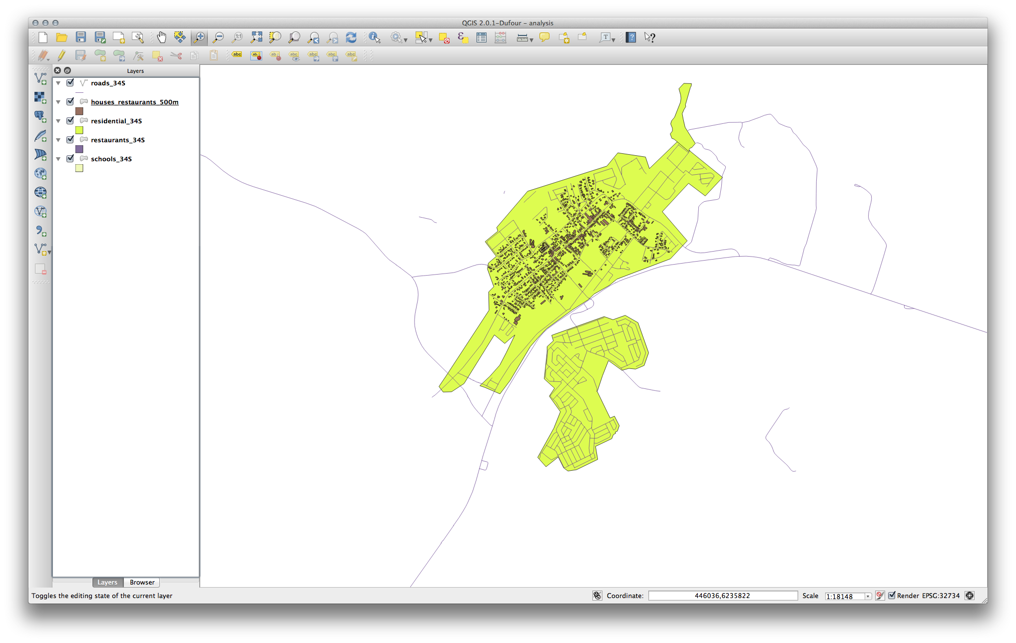
結果はこちらです:
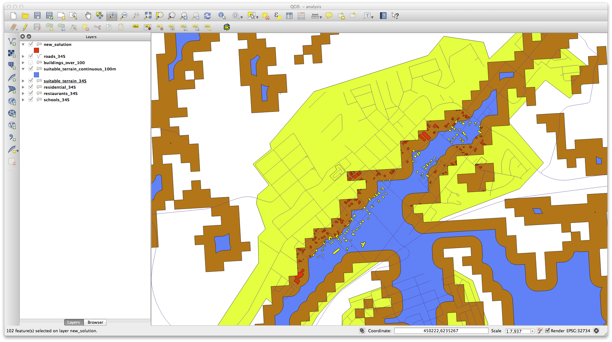
The yellow buildings are selected. Although some of the buildings fall partly outside the new suitable_terrain_continuous100m layer, they lie well within the original suitable_terrain layer and therefore meet all of our requirements.
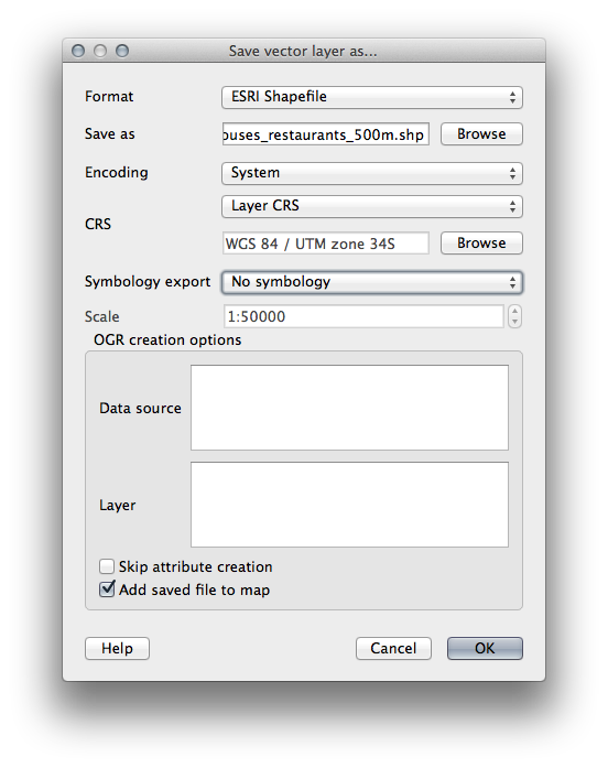
- Save the selection under exercise_data/residential_development/ as final_answer.shp.
20.12. Results For WMS
20.12.1. Adding Another WMS Layer
Your map should look like this (you may need to re-order the layers):
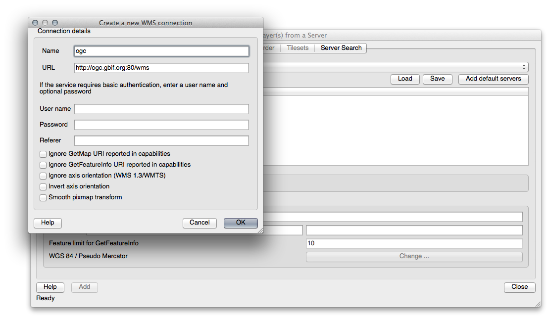
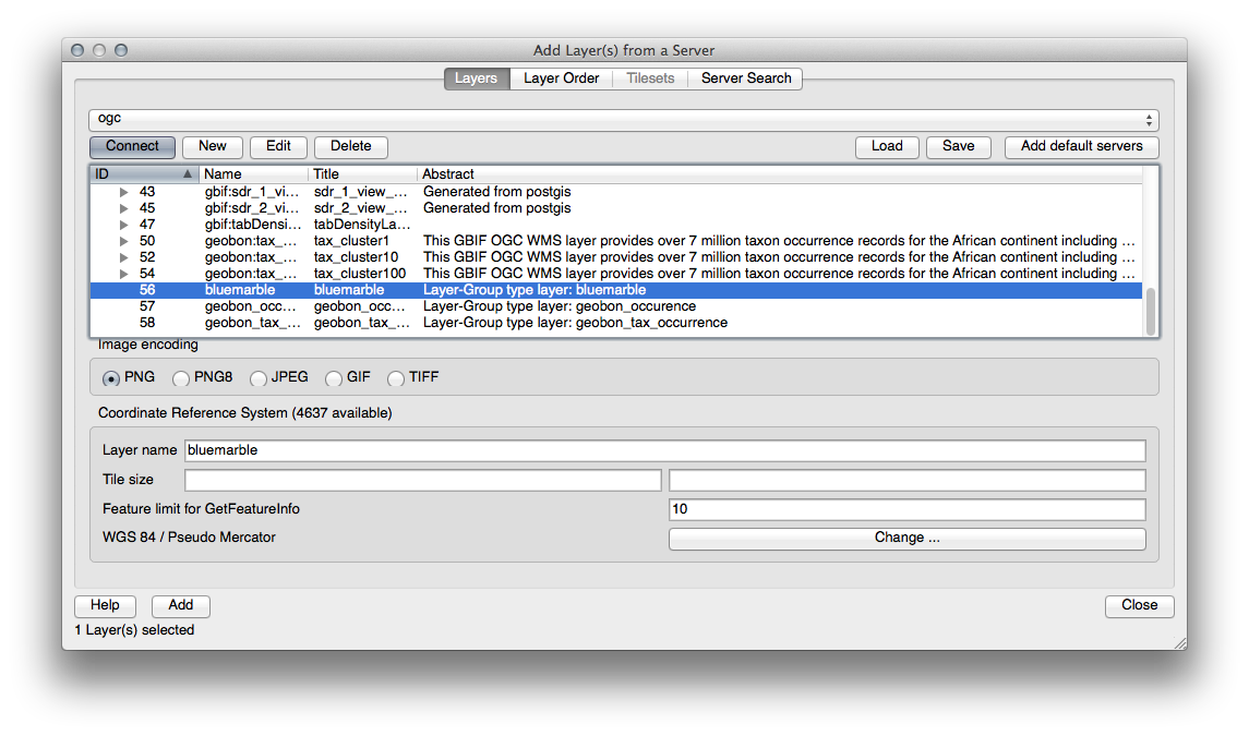
20.12.2. Adding a New WMS Server
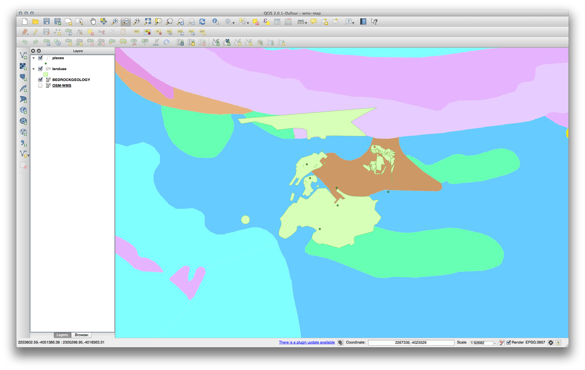
Use the same approach as before to add the new server and the appropriate layer as hosted on that server:
If you zoom into the Swellendam area, you’ll notice that this dataset has a low resolution:
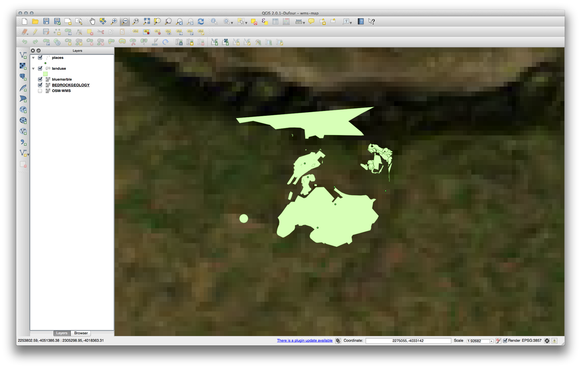
Therefore, it’s better not to use this data for the current map. The Blue Marble data is more suitable at global or national scales.
20.12.3. Finding a WMS Server
You may notice that many WMS servers are not always available. Sometimes this is temporary, sometimes it is permanent. An example of a WMS server that worked at the time of writing is the World Mineral Deposits WMS at http://apps1.gdr.nrcan.gc.ca/cgi-bin/worldmin_en-ca_ows. It does not require fees or have access constraints, and it is global. Therefore, it does satisfy the requirements. Keep in mind, however, that this is merely an example. There are many other WMS servers to choose from.
20.13. Results For Database Concepts
20.13.1. Address Table Properties
For our theoretical address table, we might want to store the following properties:
House Number
Street Name
Suburb Name
City Name
Postcode
Country
When creating the table to represent an address object, we would create columns to represent each of these properties and we would name them with SQL-compliant and possibly shortened names:
house_number
street_name
suburb
city
postcode
country
20.13.2. Normalising the People Table
The major problem with the people table is that there is a single address field which contains a person’s entire address. Thinking about our theoretical address table earlier in this lesson, we know that an address is made up of many different properties. By storing all these properties in one field, we make it much harder to update and query our data. We therefore need to split the address field into the various properties. This would give us a table which has the following structure:
id |     name      | house_no |  street_name   |    city    |   phone_no
 --+---------------+----------+----------------+------------+-----------------
 1 | Tim Sutton    |     3    | Buirski Plein  | Swellendam | 071 123 123
 2 | Horst Duester |     4    | Avenue du Roix | Geneva     | 072 121 122
ノート
In the next section, you will learn about Foreign Key relationships which could be used in this example to further improve our database’s structure.
20.13.3. Further Normalisation of the People Table
Our people table currently looks like this:
id |     name     | house_no | street_id |  phone_no
---+--------------+----------+-----------+-------------
 1 | Horst Duster |        4 |         1 | 072 121 122
The street_id column represents a ‘one to many’ relationship between the people object and the related street object, which is in the streets table.
One way to further normalise the table is to split the name field into first_name and last_name:
id | first_name | last_name  | house_no | street_id |  phone_no
---+------------+------------+----------+-----------+------------
 1 |    Horst   |   Duster   |     4    |     1     | 072 121 122
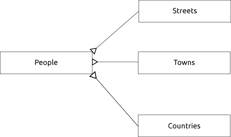
We can also create separate tables for the town or city name and country, linking them to our people table via ‘one to many’ relationships:
id | first_name | last_name | house_no | street_id | town_id | country_id
---+------------+-----------+----------+-----------+---------+------------
 1 |    Horst   |   Duster  |     4    |     1     |    2    |     1
An ER Diagram to represent this would look like this:
20.13.4. Create a People Table
The SQL required to create the correct people table is:
create table people (id serial not null primary key,
                     name varchar(50),
                     house_no int not null,
                     street_id int not null,
                     phone_no varchar null );
The schema for the table (enter \d people) looks like this:
Table "public.people"

Column     |         Type          |                      Modifiers
-----------+-----------------------+-------------------------------------
id         | integer               | not null default
           |                       | nextval('people_id_seq'::regclass)
name       | character varying(50) |
house_no   | integer               | not null
street_id  | integer               | not null
phone_no   | character varying     |
Indexes:
  "people_pkey" PRIMARY KEY, btree (id)
ノート
For illustration purposes, we have purposely omitted the fkey constraint.
20.13.5. The DROP Command
The reason the DROP command would not work in this case is because the people table has a Foreign Key constraint to the streets table. This means that dropping (or deleting) the streets table would leave the people table with references to non-existent streets data.
ノート
It is possible to ‘force’ the streets table to be deleted by using the CASCADE command, but this would also delete the people and any other table which had a relationship to the streets table. Use with caution!
20.13.6. Insert a New Street
The SQL command you should use looks like this (you can replace the street name with a name of your choice):
insert into streets (name) values ('Low Road');
20.13.7. Add a New Person With Foreign Key Relationship
Here is the correct SQL statement:
insert into streets (name) values('Main Road');
insert into people (name,house_no, street_id, phone_no)
  values ('Joe Smith',55,2,'072 882 33 21');
If you look at the streets table again (using a select statement as before), you’ll see that the id for the Main Road entry is 2.
That’s why we could merely enter the number 2 above. Even though we’re not seeing Main Road written out fully in the entry above, the database will be able to associate that with the street_id value of 2.
ノート
If you have already added a new street object, you might find that the new Main Road has an ID of 3 not 2.
20.13.8. Return Street Names
Here is the correct SQL statement you should use:
select count(people.name), streets.name
from people, streets
where people.street_id=streets.id
group by streets.name;
Result:
count |    name
------+-------------
    1 | Low Street
    2 | High street
    1 | Main Road
(3 rows)
ノート
You will notice that we have prefixed field names with table names (e.g. people.name and streets.name). This needs to be done whenever the field name is ambiguous (i.e. not unique across all tables in the database).
20.14. Results For Spatial Queries
20.14.1. The Units Used in Spatial Queries
The units being used by the example query are degrees, because the CRS that the layer is using is WGS 84. This is a Geographic CRS, which means that its units are in degrees. A Projected CRS, like the UTM projections, is in meters.
Remember that when you write a query, you need to know which units the layer’s CRS is in. This will allow you to write a query that will return the results that you expect.
20.14.2. Creating a Spatial Index
CREATE INDEX cities_geo_idx
  ON cities
  USING gist (the_geom);
20.15. Results For Geometry Construction
20.15.1. Creating Linestrings
alter table streets add column the_geom geometry;
alter table streets add constraint streets_geom_point_chk check
     (st_geometrytype(the_geom) = 'ST_LineString'::text OR the_geom IS NULL);
insert into geometry_columns values ('','public','streets','the_geom',2,4326,
     'LINESTRING');
create index streets_geo_idx
  on streets
  using gist
  (the_geom);
20.15.2. Linking Tables
delete from people;
alter table people add column city_id int not null references cities(id);
(capture cities in QGIS)
insert into people (name,house_no, street_id, phone_no, city_id, the_geom)
   values ('Faulty Towers',
           34,
           3,
           '072 812 31 28',
           1,
           'SRID=4326;POINT(33 33)');

insert into people (name,house_no, street_id, phone_no, city_id, the_geom)
   values ('IP Knightly',
           32,
           1,
           '071 812 31 28',
           1,F
           'SRID=4326;POINT(32 -34)');

insert into people (name,house_no, street_id, phone_no, city_id, the_geom)
   values ('Rusty Bedsprings',
           39,
           1,
           '071 822 31 28',
           1,
           'SRID=4326;POINT(34 -34)');
If you’re getting the following error message:
ERROR:  insert or update on table "people" violates foreign key constraint
        "people_city_id_fkey"
DETAIL: Key (city_id)=(1) is not present in table "cities".
then it means that while experimenting with creating polygons for the cities table, you must have deleted some of them and started over. Just check the entries in your cities table and use any id which exists.
20.16. Results For 簡易機能モデル
20.16.1. Populating Tables
create table cities (id serial not null primary key,
                     name varchar(50),
                     the_geom geometry not null);
 alter table cities
 add constraint cities_geom_point_chk
 check (st_geometrytype(the_geom) = 'ST_Polygon'::text );
20.16.2. Populate the Geometry_Columns Table
insert into geometry_columns values
      ('','public','cities','the_geom',2,4326,'POLYGON');
20.16.3. ジオメトリの追加
select people.name,
       streets.name as street_name,
       st_astext(people.the_geom) as geometry
from   streets, people
where  people.street_id=streets.id;
Result:
     name     | street_name |   geometry
--------------+-------------+---------------
 Roger Jones  | High street |
 Sally Norman | High street |
 Jane Smith   | Main Road   |
 Joe Bloggs   | Low Street  |
 Fault Towers | Main Road   | POINT(33 -33)
(5 rows)
ご覧のとおり、私たちの制限ではデータベースへの null の追加を認めています。