8.3. Lesson: Analiza Terenului¶

8.3.1. Follow Along: Calculul Umbrei Versanţilor¶

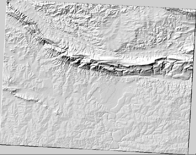
The DEM you have on your map right now does show you the elevation of the terrain, but it can sometimes seem a little abstract. It contains all the 3D information about the terrain that you need, but it doesn’t look like a 3D object. To get a better look at the terrain, it is possible to calculate a hillshade, which is a raster that maps the terrain using light and shadow to create a 3D-looking image.

Pentru a lucra cu DEM-uri, ar trebui să utilizați instrumentele de analiză all-in-one DEM (Terrain models) din QGIS.

• Faceți clic pe elementul de meniu Raster ‣ Analysis ‣ DEM (Terrain models).

• În caseta de dialog care apare, asigurați-vă că Fișierul de intrare este stratul DEM.

• Setați Fișierul de ieșire ca hillshade.tif, în directorul exercise_data/residential_development/.

• De asemenea, asigurați-vă că pentru opțiunea Mode s-a ales Hillshade.

• Bifaţi caseta de lângă Load into canvas when finished.

• Puteți lăsa toate celelalte opțiuni neschimbate.

• Clic pe OK, pentru a genera umbra versanților.

• Atunci când vi se spune că prelucrarea este finalizată, faceți clic pe OK, pentru închiderea mesajului.

• Faceți clic pe Close din dialogul principal al DEM (Terrain models).

Aveți acum un nou strat denumit hillshade, care arată astfel:

That looks nice and 3D, but can we improve on this? On its own, the hillshade looks like a plaster cast. Can’t we use it together with our other, more colorful rasters somehow? Of course we can, by using the hillshade as an overlay.

8.3.2. Follow Along: Folosirea Umbrei Versanților pentru Suprapunere¶

Umbra versanților poate furniza informații foarte utile despre lumina solară, la un moment dat al zilei. Ea poate fi, de asemenea, utilizată în scopuri estetice, pentru a face harta să arate mai bine. Cheia pentru acest lucru este setarea reliefului de a fi în cea mai mare parte transparent.

• Schimbarea simbologiei DEM-ului original pentru utilizarea schemei guilabel:Pseudocolor, ca și în exercițiul anterior.

• Ascundeți toate straturile, cu excepția straturilor DEM și hillshade.

• Efectuați clic pe DEM și glisați-l sub stratul hillshade din Lista straturilor.

• Set the hillshade layer to be transparent by opening its Layer Properties and go to the Transparency tab.

• Setați Transparența globală la 50%:

• Clic OK în dialogul Layer Properties. Veți obține un rezultat ca aceasta:

  

• Switch the hillshade layer off and back on in the Layers list to see the difference it makes.

Using a hillshade in this way, it’s possible to enhance the topography of the landscape. If the effect doesn’t seem strong enough to you, you can change the transparency of the hillshade layer; but of course, the brighter the hillshade becomes, the dimmer the colors behind it will be. You will need to find a balance that works for you.

Amintiți-vă să salvați harta, după ce ați definitivat.

8.3.3. Follow Along: Calculul Pantei¶

În cazul unui teren, este util să-i cunoașteți panta. Dacă, de exemplu, doriți să construiți niște case pe un teren, atunci este necesar ca un teren să fie relativ plat.

Pentru a face acest lucru, trebuie să folosiți modul Slope al instrumentului DEM (Terrain models).

• Deschideți instrumentul ca și înainte.

• Selectați Slope pentru opțiunea Mode:

  

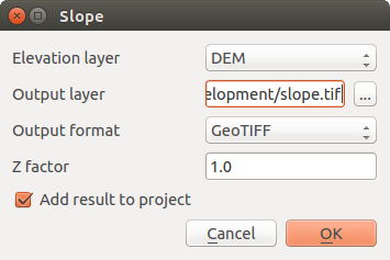
• Setați locația pentru salvare exercise_data/residential_development/slope.tif

• Bifați caseta Load into canvas....

• Click OK and close the dialogs when processing is complete, and click Close to close the dialog. You’ll see a new raster loaded into your map.

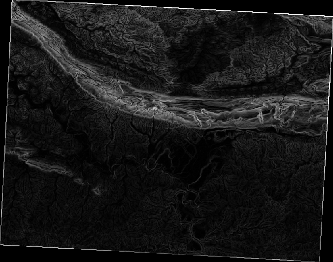
• With the new raster selected in the Layers list, click the Stretch Histogram to Full Dataset button. Now you’ll see the slope of the terrain, with black pixels being flat terrain and white pixels, steep terrain:

  

8.3.4. Try Yourself Calculați aspectul¶

The aspect of terrain refers to the direction it’s facing in. Since this study is taking place in the Southern Hemisphere, properties should ideally be built on a north-facing slope so that they can remain in the sunlight.

• Use the Aspect mode of the DEM (Terain models) tool to calculate the aspect of the terrain.

Verificați-vă rezultatele

8.3.5. Follow Along: Folosirea Calculatorului Raster¶

Think back to the estate agent problem, which we last addressed in the Vector Analysis lesson. Let’s imagine that the buyers now wish to purchase a building and build a smaller cottage on the property. In the Southern Hemisphere, we know that an ideal plot for development needs to have areas on it that are north-facing, and with a slope of less than five degrees. But if the slope is less than 2 degrees, then the aspect doesn’t matter.

Fortunately, you already have rasters showing you the slope as well as the aspect, but you have no way of knowing where both conditions are satisfied at once. How could this analysis be done?

Răspunsul se află cu ajutorul: Calculatorului raster.

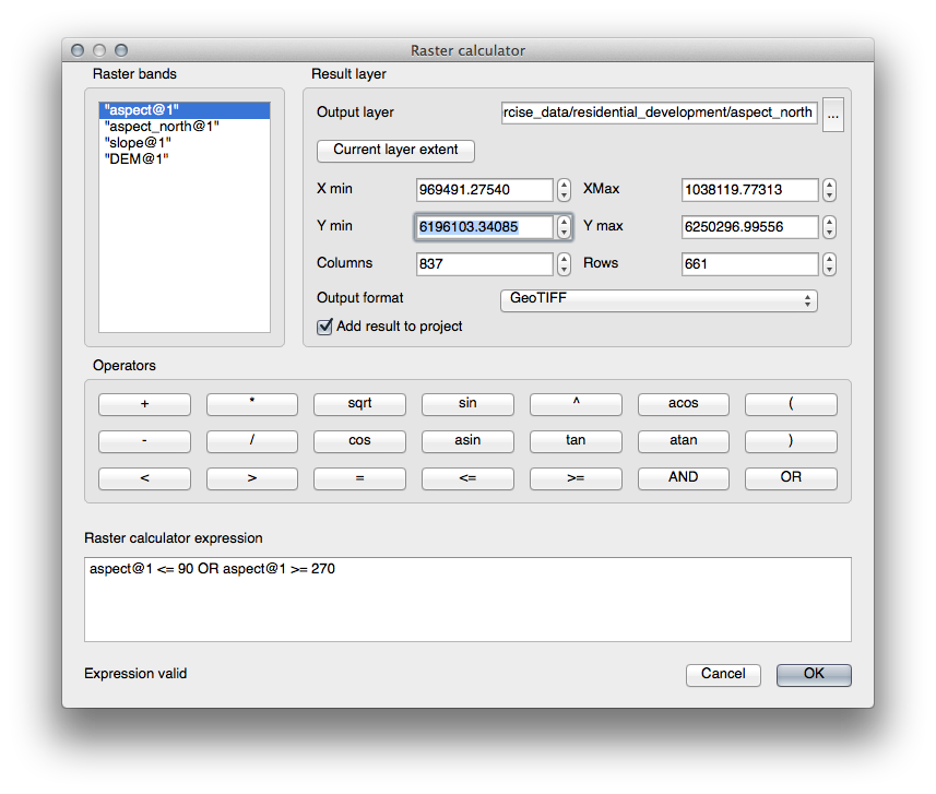
• Faceți clic pe Raster > Raster calculator... pentru a deschide acest instrument.

• To make use of the aspect dataset, double-click on the item aspect@1 in the Raster bands list on the left. It will appear in the Raster calculator expression text field below.

North is at 0 (zero) degrees, so for the terrain to face north, its aspect needs to be greater than 270 degrees and less than 90 degrees.

• În câmpul Expresiei calculatorului raster, introduceți:

  aspect@1 <= 90 OR aspect@1 >= 270

• Setați ca fișierul de ieșire aspect_north.tif din directorul exercise_data/residential_development/.

• Asigurați-vă că este selectată caseta Add result to project.

• Faceți clic pe Ok pentru a începe procesarea.

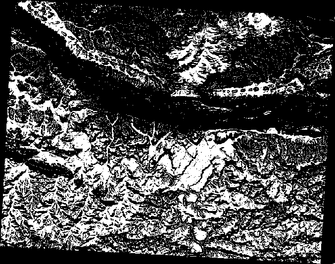
Rezultatul va fi acesta:

8.3.6. Try Yourself¶

Acum, că ați definitivat aspectul, crea două noi analize separate, ale stratului DEM.

• Prima va fi de a identifica toate zonele unde panta este mai mică sau egală cu 2 grade.

• A doua este similară, dar panta trebuie să fie mai mică sau egală cu 5 grade.

• Salvați-le sub exercise_data/residential_development/ ca slope_lte2.tif și slope_lte5.tif.

Verificați-vă rezultatele

8.3.7. Follow Along: Combinarea Rezultatelor Analizei Raster¶

Acum aveți trei noi Analize Raster ale stratului DEM:

• aspect_north: terenul orientat spre nord

• slope_lte2: panta este la, sau sub, 2 grade

• slope_lte5: panta este la, sau sub, 5 grade

Where the conditions of these layers are met, they are equal to 1. Elsewhere, they are equal to 0. Therefore, if you multiply one of these rasters by another one, you will get the areas where both of them are equal to 1.

The conditions to be met are: at or below 5 degrees of slope, the terrain must face north; but at or below 2 degrees of slope, the direction that the terrain faces in does not matter.

Therefore, you need to find areas where the slope is at or below 5 degrees AND the terrain is facing north; OR the slope is at or below 2 degrees. Such terrain would be suitable for development.

Pentru a calcula zonele care îndeplinesc aceste criterii:

• Deschideți iarăși Calculatorul raster.

• Folosiți Raster bands, butoanelor Operatorilor, și tastatura dvs. pentru a construi această expresie din zona de text a Calculatorului de expresii raster:

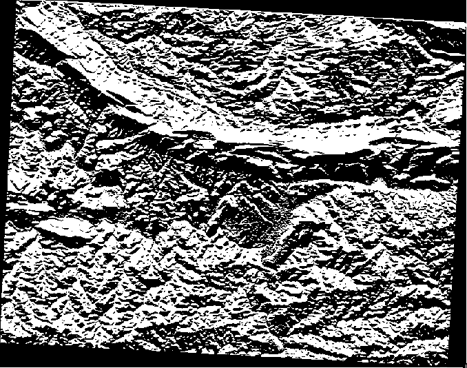
  ( aspect_north@1 = 1 AND slope_lte5@1 = 1 )  OR slope_lte2@1 = 1

• Salvați rezultatul în exercise_data/residential_development/ ca all_conditions.tif.

• Clic OK în dialogul Calculatorul raster. Rezultatele dvs.:

  

8.3.8. Follow Along: Simplificarea Rasterului¶

As you can see from the image above, the combined analysis has left us with many, very small areas where the conditions are met. But these aren’t really useful for our analysis, since they’re too small to build anything on. Let’s get rid of all these tiny unusable areas.

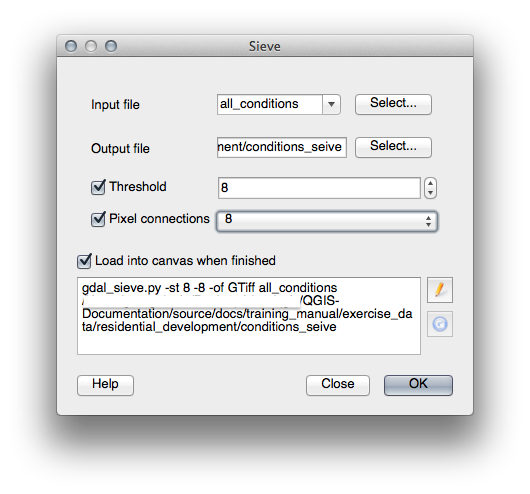
• Deschideți instrumentul Sieve (Raster ‣ Analysis ‣ Sieve).

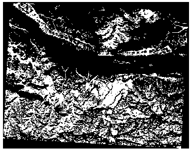
• Setați Fișierul de intrare pe all_conditions, iar Fișierul de ieșire pe all_conditions_sieve.tif (de sub exercise_data/residential_development/).

• Setați valorile Threshold și Pixel connections pe 8, apoi rulați instrumentul.

O dată de s-a încheiat prelucrarea, noul strat se va încărca în canevas. Dar atunci când încercați să utilizați instrumentul de întindere a histogramei pentru a vizualiza datele, se întâmplă următorul lucru:

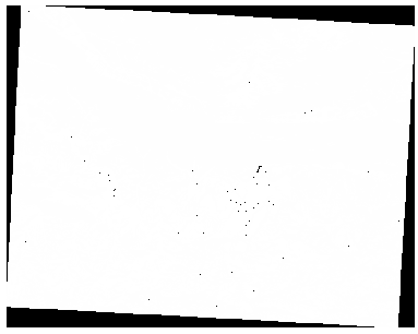
Ce se întâmplă? Răspunsul se află în metadatele noului fișier raster.

• Vizualizarea metadatelor de sub fila Metadata, a dialogului Layer Properties. Uitați-vă în secțiunea Properties din partea de jos.

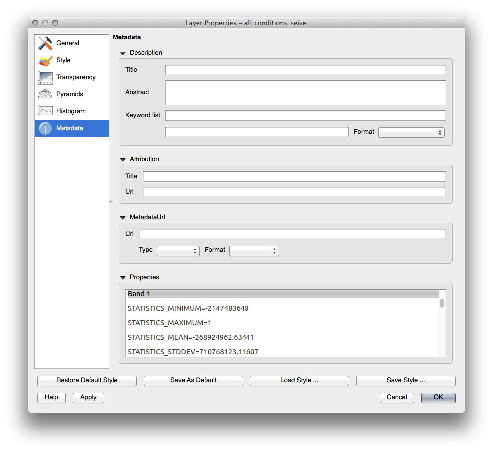
Whereas this raster, like the one it’s derived from, should only feature the values 1 and 0, it has the STATISTICS_MINIMUM value of a very large negative number. Investigation of the data shows that this number acts as a null value. Since we’re only after areas that weren’t filtered out, let’s set these null values to zero.

• Deschideți iarăși Calculatorul raster, și construiți această expresie:

  (all_conditions_sieve@1 <= 0) = 0

  Acest lucru va menține toate valorile existente la zero, în timp ce, de asemenea, se pun pe zero numerele negative; ceea ce va lăsa intacte toate zonele cu valoarea 1.

• Salvați rezultatul în exercise_data/residential_development/ ca all_conditions_simple.tif.

Rezultatul dvs. arată în felul următor:

This is what was expected: a simplified version of the earlier results. Remember that if the results you get from a tool aren’t what you expected, viewing the metadata (and vector attributes, if applicable) can prove essential to solving the problem.

8.3.9. In Conclusion¶

You’ve seen how to derive all kinds of analysis products from a DEM. These include hillshade, slope and aspect calculations. You’ve also seen how to use the raster calculator to further analyze and combine these results.

8.3.10. What’s Next?¶

Now you have two analyses: the vector analysis which shows you the potentially suitable plots, and the raster analysis that shows you the potentially suitable terrain. How can these be combined to arrive at a final result for this problem? That’s the topic for the next lesson, starting in the next module.