17.16. Analize hidrologice
Note
În această lecție, vom efectua unele analize hidrologice. Această analiză va fi utilizată în unele din următoarele lecții, deoarece constituie un exemplu foarte bun de analiză a fluxului de lucru, pe care o vom folosi pentru a demonstra unele caracteristici avansate.
În această lecție, vom face unele analize hidrologice. Începând cu un DEM, vom extrage o rețea de canale, vom delimita bazinele hidrografice și vom calcula unele statistici.
Primul lucru este de a încărca proiectul cu datele lecției, care conține doar un DEM.
The first module to execute is Catchment area. You can use anyone of the others named Catchment area. They have different algorithms underneath, but the results are basically the same.
Selectați DEM-ul din câmpul Elevație, lăsând valorile implicite pentru restul parametrilor.
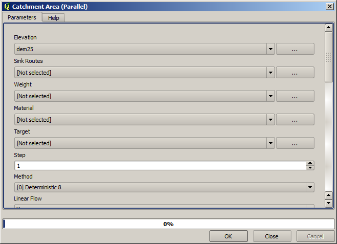
Unii algoritmi calculează multe straturi, dar Catchment Area este cel pe care dorim să-l folosim.
Puteți scăpa de celelalte, dacă doriți.
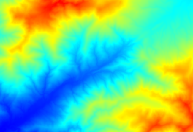
Randarea stratului nu este foarte informativă.

To know why, you can have a look at the histogram and you will see that values are not evenly distributed (there are a few cells with very high value, those corresponding to the channel network). Calculating the logarithm of the catchment area value yields a layer that conveys much more information (you can do it using the raster calculator).

The catchment area (also known as flow accumulation), can be used to set a threshold for channel initiation. This can be done using the Channel network algorithm. Here is how you have to set it up (note the Initiation threshold Greater than 10.000.000).
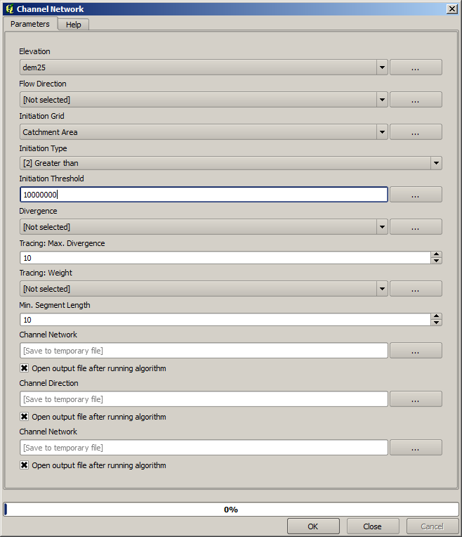
Utilizați stratul original al bazinului hidrografic, nu cel logaritmic. Acela folosește doar pentru randare.
If you increase the Initiation threshold value, you will get a more sparse channel network. If you decrease it, you will get a denser one. With the proposed value, this is what you get.

Imaginea de mai sus prezintă doar stratul vectorul rezultat și DEM-ul, dar ar trebui să fie și unul raster, cu aceeași rețea de canale. Rasterul va fi, de fapt, cel pe care îl vom folosi.
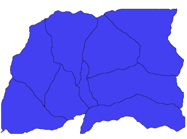
Now, we will use the Watersheds basins algorithm to delineate the subbasins corresponding to that channel network, using as outlet points all the junctions in it. Here is how you have to set the corresponding parameters dialog.

Acesta veți obține.
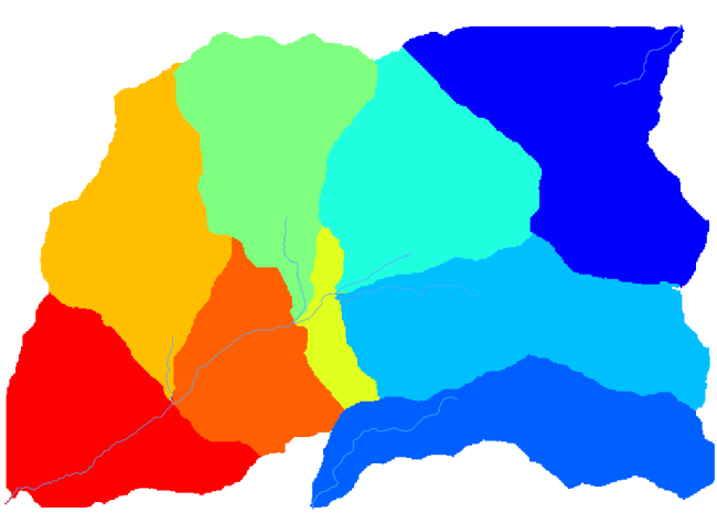
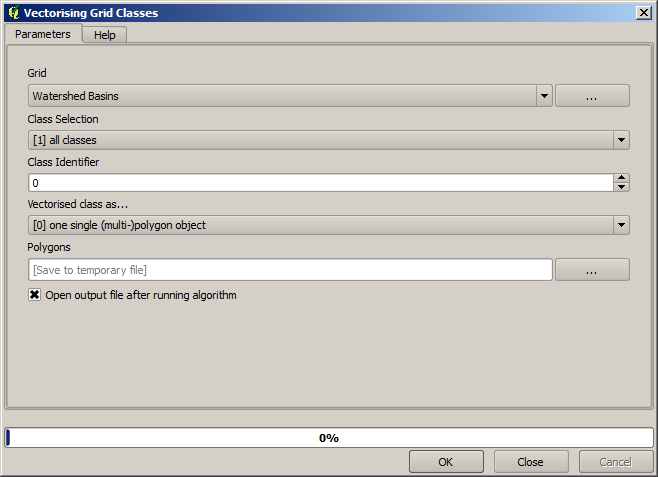
Acesta este rasterul rezultat. Puteți să-l vectorizați folosind algoritmul Vectorizarea claselor grilei.
Now, let’s try to compute statistics about the elevation values in one of the subbasins. The idea is to have a layer that just represents the elevation within that subbasin and then pass it to the module that calculates those statistics.
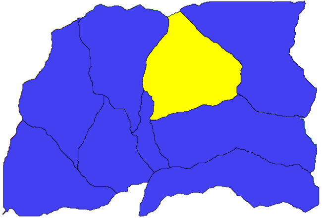
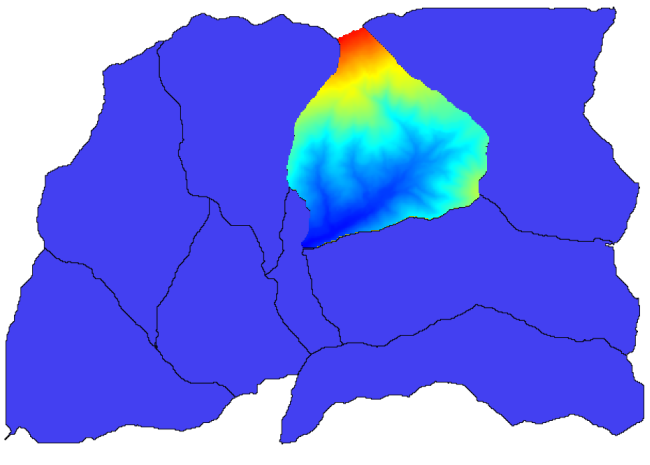
First, let’s clip the original DEM with the polygon representing a subbasin. We will use the Clip grid with polygon algorithm. If we select a single subbasin polygon and then call the clipping algorithm, we can clip the DEM to the area covered by that polygon, since the algorithm is aware of the selection.
Selectați un poligon,
și apelați algoritmul de tăiere cu următorii parametri:
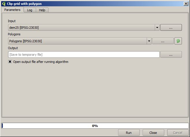
Elementul selectat în câmpul de introducere este, desigur, DEM-ul pe care vrem să-l decupăm.
Veți obține ceva de genul acesta.
Acest strat este gata de a fi utilizat in algoritmul Raster layer statistics.
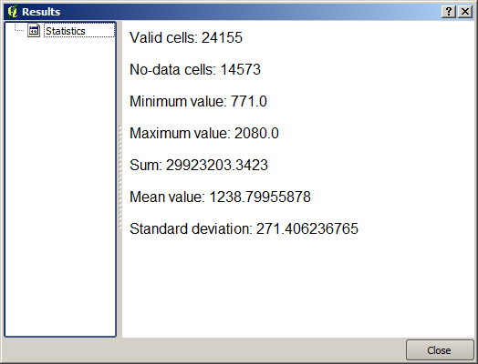
Statisticile rezultate sunt următoarele.
Vom folosi și în alte lecții atât procedura de calcule a bazinului, cât și calcularea statisticilor, pentru a afla cum ne pot ajuta alte elemente la automatizarea amândurora, cât și pentru a lucra mai eficient.