14.5. Lesson: Planul de Eșantionare Sistematică
You have already digitized a set of polygons that represent the forest stands, but you don’t have information about the forest just yet. For that purpose you can design a survey to inventory the whole forest area and then estimate its parameters. In this lesson you will create a systematic set of sampling plots.
When you start planning your forest inventory it is important to clearly define the objectives, the types of sample plots that will be used, and the data that will be collected to achieve the objectives. For each individual case, those will depend on the type of forest and the management purpose; and should be carefully planned by someone with forestry knowledge. In this lesson, you will implement a theoretical inventory based on a systematic sampling plot design.
Scopul acestei lecții: De a crea un grafic de eșantionare sistematic, proiectat pentru o vedere de ansamblu a zonei de pădure.
14.5.1. Inventarierea Pădurii
There are several methods to inventory forests, each of them suiting different purposes and conditions. For example, one very accurate way to inventory a forest (if you consider only tree species) would be to visit the forest and make a list of every tree and their characteristics. As you can imagine this is not commonly applicable except for some small areas or some special situations.
The most common way to find out about a forest is by sampling it, that is, taking measurements in different locations at the forest and generalizing that information to the whole forest. These measurements are often made in sample plots that are smaller forest areas that can be easily measured. The sample plots can be of any size (for ex. 50 m2, 0.5 ha) and form (for ex. circular, rectangular, variable size), and can be located in the forest in different ways (for ex. randomly, systematically, along lines). The size, form and location of the sample plots are usually decided following statistical, economical and practical considerations. If you have no forestry knowledge, you might be interested in reading this Wikipedia article.
14.5.2. Lesson: Implementarea unui Plan de Eșantionare Sistematică
For the forest you are working with, the manager has decided that a systematic sampling design is the most appropriate for this forest and has decided that a fixed distance of 80 meters between the sample plots and sampling lines will yield reliable results (for this case, +- 5% average error at a probability of 68%). Variable size plots has been decided to be the most effective method for this inventory, for growing and mature stands, but a 4 meters fixed radius plots will be used for seedling stands.
În practică, trebuie pur și simplu să reprezentăm parcelele eșantion ca puncte care vor fi folosite ulterior de către echipele din teren:
Deschideți proiectul
digitizing_2012.qgsEliminați toate straturile, cu excepția
forest_stands_2012.Salvați proiectul dumneavoastră ca
forest_inventory.qgs
Acum trebuie să creați o rețea dreptunghiulară de puncte separate, aflate la 80 de metri unul de altul:
Deschideți Vector ‣ Research Tools ‣ Regular points.
În definițiile Ariei, selectați Input Boundary Layer.
Iar ca și strat de intrare setați
forest_stands_2012.În setările de Spațiere a Grilei, selectați Folosirea acestei spațieri între puncte și stabiliți-o la
80.Salvați rezultatul ca
systematic_plots.shp, în folderulforestry\sampling\.Bifați caseta Add result to canvas.
Clic pe OK
Note
The suggested Regular points creates the systematic points starting in the corner upper-left corner of the extent of the selected polygon layer. If you want to add some randomness to this regular points, you could use a randomly calculated number between 0 and 80 (80 is the distance between our points), and then write it as the Initial inset from corner (LH side) parameter in the tool’s dialog.
You notice that the tool has used the whole extent of your stands layer to generate a rectangular grid of points. But you are only interested on those points that are actually inside your forest area (see the images below):
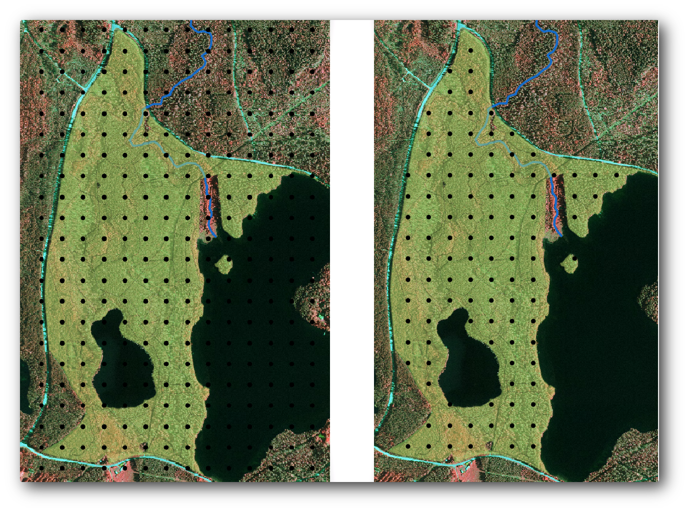
Deschideți Vector ‣ Geoprocessing Tools ‣ Clip.
Selectați
systematic_plotsca Strat vectorial de intrare.Setați
forest_stands_2012ca și Strat de decupare.Salvați rezultatul ca și
systematic_plots_clip.shp.Bifați caseta Add result to canvas.
Clic pe OK
You have now the points that the field teams will use to navigate to the designed sample plots locations. You can still prepare these points so that they are more useful for the field work. At the least you will have to add meaningful names for the points and export them to a format that can be used in their GPS devices.
Lets start with the naming of the sample plots. If you check the Attribute table for the plots inside the forest area, you can see that you have the default id field automatically generated by the Regular points tool. Label the points to see them in the map and consider if you could use those numbers as part of your sample plot naming:
Deschideți Layer Properties –> Labels pentru
systematic_plots_clip.Bifați Label this layer with, apoi selectați câmpul
ID.- Go to the Buffer options and check the Draw text buffer, set the Size to
1. Clic pe OK
Now look at the labels on your map. You can see that the points have been created and numbered first West to East and then North to South. If you look at the attribute table again, you will notice that the order in the table is following also that pattern. Unless you would have a reason to name the sample plots in a different way, naming them in a West-East/North-South fashion follows a logical order and is a good option.
Note
If you would like to order or name them in a different way, you could use a spreadsheet to be able to order and combine rows and columns in any different way.
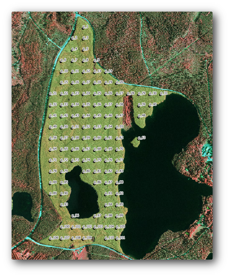
Nevertheless, the number values in the id field are not so good. It would be better if the naming would be something like p_1, p_2.... You can create a new column for the systematic_plots_clip layer:
Mergeți la Tabelul de atribute pentru
systematic_plots_clip.Activați modul de editare.
Deschideți Calculatorul de câmpuri, apoi denumiți noua coloană
Plot_id.Setați Output field type la
Text (string).- In the Expression field, write, copy or construct this formula
concat('P_', $rownum ). Remember that you can also double click on the elements inside the Function list. Theconcatfunction can be found under String and the$rownumparameter can be found under Record. Clic pe OK
Dezactivați modul de editare și salvați modificările.
Now you have a new column with plot names that are meaningful to you. For the systematic_plots_clip layer, change the field used for labeling to your new Plot_id field.
14.5.3.  Follow Along: Exportați Graficele în format GPX
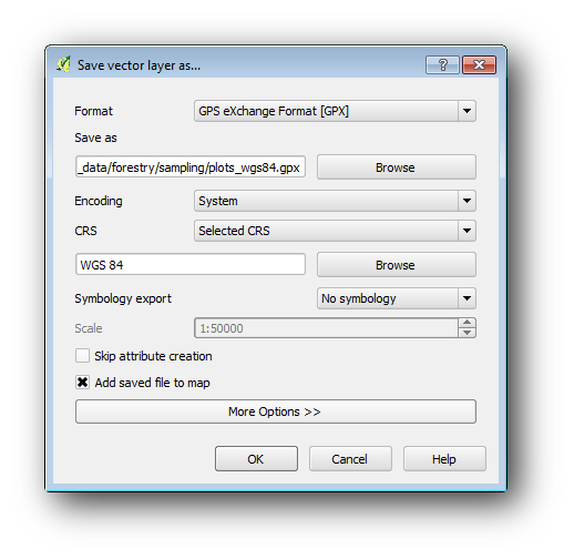
The field teams will be probably using a GPS device to locate the sample plots you planned. The next step is to export the points you created to a format that your GPS can read. QGIS allows you to save your point and line vector data in GPS eXchange Format (GPX)<http://en.wikipedia.org/wiki/GPS_Exchange_Format>, which is an standard GPS data format that can be read by most of the specialized software. You need to be careful with selecting the CRS when you save your data:
Clic dreapta pe
systematic_plots_clip, apoi selectați Save as.În Format selectați GPS eXchange Format [GPX].
Salvați rezultatul ca
plots_wgs84.gpx.În CRS alegeți CRS-ul Selectat.
Alegeți
WGS 84 (EPSG:4326).
..note:: The GPX format accepts only this CRS, if you select a different one, QGIS will give no error but you will get an empty file.
Clic pe OK
- In the dialog that opens, select only the
waypointslayer (the rest of the layers are empty).
The inventory sample plots are now in a standard format that can be managed by most of the GPS software. The field teams can now upload the locations of the sample plots to their devices. That would be done by using the specific devices own software and the plots_wgs84.gpx file you just saved. Other option would be to use the GPS Tools plugin but it would most likely involve setting the tool to work with your specific GPS device. If you are working with your own data and want to see how the tool works you can find out information about it in the section Working with GPS Data in the QGIS User Manual.
Salvați acum proiectul dvs. QGIS.
14.5.4. In Conclusion
You just saw how easily you can create a systematic sampling design to be used in a forest inventory. Creating other types of sampling designs will involve the use of different tools within QGIS, spreadsheets or scripting to calculate the coordinates of the sample plots, but the general idea remains the same.
14.5.5. What’s Next?
In the next lesson you will see how to use the Atlas capabilities in QGIS to automatically generate detailed maps that the field teams will be using to navigate to the sample plots assigned to them.